本来想着放在笔记后面,后来发现好像问题有点多…决定新开一篇文章来写
hw1
https://www.kaggle.com/c/ml2019spring-hw1/overview
作业说明
我一开始做了一个非常naive的model,反正分开处理,Python用的也不是很熟练,就当练代码了
一开始没用AdaGrad,发现Learning Rate真的很难设置
如果数据量小,那么Learning Rate应该大一些,如果数据量大,那就得小一些了,这个都是相对的
如果数据本身小,那么初始值就没那么重要,如果本身大的话,那初始值就需要自己手动设置一下了
举个第一个的栗子,如果一开始初始值都设成0,12960条数据,一开始得到的Loss就有51361098.87099994,Learning Rate我设成了1e-8,得到的结果还越来越大…
当我把数据量调小一点,比如20条这个样子,还是有点用的…Learning Rate = 1e-6,迭代50次大概能得到一个不错的结果…
实测1e-9,1e-12时有点用了…
我忽然有个大胆的想法…如果前面变化大点后面变化小点是不是很科学,可以飞快接近结果
p.s. Python的输出调试真的不好用…不如c++的#define debug(x) cout<<#x<<"="<<x<<endl,可能我还没get到该技能
原来只需要预测PM2.5就行了,那我直接写全得了
一开始Loss=4231600.00,最后313187.27500353276
现在我不是很清楚要什么时候结束…所以先直接计次循环了
先在这保存一下代码…之后改成AdaGrad
果然这个naive的程序得到了private:9.66107 public:8.18926的高分,我觉得以后应该把训练的模块和输出模块分开来写,不然必须训练一次才能输出233
第一次训练出来的w和b
1 | w = [0.02560433358938389, 0.012801930896077247, 0.004710981594648449, 0.005885507375027003, 0.009942499746330985, 0.026670961533262413, -0.0010603121145215564, 0.25976948883940576, 0.6202885065990642] |
1 | import numpy as np |
其实我觉得浮点数精度带来的误差还是很大的…
今天跑不完了,明早起来再跑吧233
1 | import numpy as np |
总共跑了大概30min,然后得到了一个结果226303.2859914291,得到的w和b在下面,得到的分数是private:7.29680 public:6.02679,也差不多是我这种乱搞做法的比较好的结果了吧1
2w = [-0.01196089473848148, -0.0002154942523566853, 0.15614885717614674, -0.18703390611436793, -0.028484991059330843, 0.46031602604586386, -0.5230520726349329, 0.013331313987351568, 1.091108574289711]
b = 0.15907341031251657
我发现那个助教做Demo的时候也是计次…
AdaGrad 有进步但是不太大private:7.24162 public:5.93032
我发现Learning Rate的初始值还是很重要的,不然第一次偏差太大,后面跑回来就比较慢了
我又在这基础上Train了一下,private:7.24797 public:5.92997,分数反而下降了…
不解挠头,我好像不知道怎么变得更好了…
我觉得吧…可能是多加些参数了,把其他的条件考虑进去再加上二次项
1 | import numpy as np |
哇哦 果然,考虑了二次项,就Training了一次,从0开始,虽然得到的loss有249940.5819514999,但是得到的结果就比之前好得多private:7.19917 public:6.21872
惊了第二次private:6.64656 public:6.05368,直接过了strong baseline,进前30了…
第三次private:6.48045 public:5.98424,嗯,这个作业就先这样吧…继续看看然后搞后面的了
1 | # train once |
1 | import numpy as np |
加了三次方,感觉要Overfitting…
哦 结果变得肥肠爆炸…
1 | import numpy as np |
hw2
https://www.kaggle.com/c/ml2019spring-hw2
作业说明
这就是一个Binary Classification,直接用X_train提出的特征就可以了
Probabilistic Generateive Model
假设是高斯分布来算的,所以不需要训练,秒出结果,得分也不太高private:0.76047 public:0.76707
也不知道是不是我写挂了…
没错是我写挂了,这全是0吧…
ps.手写矩阵运算好麻烦啊,虽然也不长,但是种类太多,感觉不如C++方便,可能我都写C++写惯了,抽时间看一下numpy好了
probabilistic_generateive_model.py1
2
3
4
5
6
7
8
9
10
11
12
13
14
15
16
17
18
19
20
21
22
23
24
25
26
27
28
29
30
31
32
33
34
35
36
37
38
39
40
41
42
43
44
45
46
47
48
49
50
51
52
53
54
55
56
57
58
59
60
61
62
63
64
65
66
67
68
69
70
71
72
73
74
75
76
77
78
79
80
81
82
83
84
85
86
87
88
89
90
91
92
93
94
95
96
97
98
99
100
101
102
103
104
105
106
107
108
109
110
111
112
113
114
115
116
117
118
119
120
121
122
123
124
125
126
127
128
129
130
131
132
133
134
135
136
137
138
139
140
141
142
143
144
145
146
147
148
149
150
151
152
153
154
155
156
157
158
159
160
161
162
163
164
165
166
167
168import numpy as np
from math import pi, log, exp
file_x = open('X_train', 'r')
file_y = open('Y_train', 'r')
file_xt = open('X_test', 'r')
file_yt = open('Y_test', 'w')
#x_train = y_train = x_test = []
#mu1 = mu2 = sigm = []
def deal_data(x):
for i in range(0, len(x)):
x[i]=x[i].split(',')
for j in range(0, len(x[i])):
x[i][j]=int(x[i][j])
def load_data():
global x_train, y_train, x_test
x_train = file_x.readlines()[1:]
y_train = file_y.readlines()[1:]
x_test = file_xt.readlines()[1:]
deal_data(x_train)
deal_data(y_train)
deal_data(x_test)
def mult(a, b):
c = []
for i in range(len(a)):
c.append([])
for j in range(len(b[0])):
c[i].append(0)
for i in range(len(a)):
for j in range(len(b)):
for k in range(len(b[0])):
c[i][k] += a[i][j]*b[j][k]
return c
def mult_num(a, b):
c = []
for i in range(len(a)):
c.append([])
for j in range(len(a[i])):
c[i].append(a[i][j]*b)
return c
def add(a, b):
c = []
for i in range(len(a)):
c.append([])
for j in range(len(a[0])):
c[i].append(0)
for i in range(len(a)):
for j in range(len(a[0])):
c[i][j] = a[i][j]+b[i][j]
return c
def transpose(a):
c = []
for i in range(len(a[0])):
c.append([])
for j in range(len(a)):
c[i].append(a[j][i])
return c
def train():
global x_train, y_train, x_test
global n, n0, n1, dim, mu0, mu1, sigm, sigm0, sigm1, w, b
n = len(y_train)
n0 = n1 = 0
dim = len(x_train[0])
mu0 = []
mu1 = []
for i in range(dim):
mu0.append(0)
mu1.append(0)
for i in range(n):
if y_train[i][0] == 0:
n0+=1
for j in range(dim):
mu0[j] += x_train[i][j]
else:
n1+=1
for j in range(dim):
mu1[j] += x_train[i][j]
for i in range(dim):
mu0[i] /= n0
mu1[i] /= n1
sigm0 = 0
sigm1 = 0
# for i in range(dim):
# sigm0.append(0)
# sigm1.append(0)
for i in range(n):
if y_train[i][0] == 0:
for j in range(dim):
sigm0+=(x_train[i][j]-mu0[j])**2
else:
for j in range(dim):
sigm1+=(x_train[i][j]-mu1[j])**2
sigm0 /= n0
sigm1 /= n1
sigm = n0/(n0+n1)*sigm0 + n1/(n0+n1)*sigm1
#change to vector
w = []
for i in range(dim):
w.append((mu0[i]-mu1[i])/sigm)
for i in range(dim):
mu0[i] = [mu0[i]]
mu1[i] = [mu1[i]]
b0 = mult_num(mult(transpose(mu0), mu0), -0.5/sigm)
b1 = mult_num(mult(transpose(mu1), mu1), 0.5/sigm)
b = add(b0, b1)
b = b[0][0]+log(n0/n1)
# print(b)
# for i in range(dim):
# sigm0[i] /= n0
# sigm1[i] /= n1
def sigmoid(z):
return 1/(1+exp(-z))
def get_probability(x):
global w, b
z=0
for i in range(dim):
z += w[i]*x[i]
z += b
return sigmoid(z)
def get_predict(x):
if get_probability(x)>0.5:
return 0
else:
return 1
def test():
print('id,label', file=file_yt)
for i in range(len(x_test)):
print(i+1, get_predict(x_test[i]),sep=',', file=file_yt)
def main():
load_data()
print('load_data() ok')
train()
print('train() ok')
test()
print('test() ok')
if __name__ == '__main__':
main()
Logistic Regression Model
设$s(x)=\frac{1}{1+e^{-x}}$,那么$s’(x)=s(x)(1-s(x))$,反过来证明很简单,正推求导还是有些麻烦的
这个1w数据,又有很多浮点运算…实在是难顶…好慢…
哎,写了个Logistic Regression,train来train去,0还是太少了,我佛啦
我发现它每个几个就会出现一次结果非常糟的情况…
参考了下别人的代码魔改了一发,就是加上了AdaGrad,然后求偏微分的时候除总数,再加上Regularization
哇! 我懂了!
有个肥肠肥肠肥肠肥肠肥肠肥肠肥肠肥肠肥肠重要的数据处理就是把一些范围肥肠大的数据范围变小,就除均值就可以了,在这里,有第0,1,3,4,5有关年龄,收入支出的部分范围特别大,把他范围缩小,然后再train就不会出现之前那样每个几个就会出现一次结果非常糟的情况了,train 30次就能得到private:0.84363 public:0.84656
最高也就private: 0.85345 public:0.85356
1 | import numpy as np |
我又修改了一下处理数据那部分,把范围大的变成$\frac{x-\min\{x\}}{\max\{x\}-\min\{x\}}$
结果稍差了一丢丢private:0.84903 public:0.85282
不管了…看后面的了
1 | def deal_col(x, a, xt): |
hw3
https://www.kaggle.com/c/ml2019spring-hw3
作业说明
Model
要做的是一个人脸表情的分类
数据处理的部分用了好长时间,主要是显式循环太致命了…我还不太会处理csv,所以直接暴力读文件处理了
这是最一开始写的,得到的output是这样1
2
3
4
5
6
7
8
9
10
11
12
13
14
15
16
17
18
19
20
21
22
23
24
25
26
27
28
29
30
31
32
33
34
35
36
37
38
39
40
41
42
43
44
45
46
47
48Epoch 1/20
2019-07-30 23:58:40.386315: I tensorflow/core/platform/cpu_feature_guard.cc:142] Your CPU supports instructions that this TensorFlow binary was not compiled to use: AVX2 FMA
2019-07-30 23:58:40.410366: I tensorflow/core/platform/profile_utils/cpu_utils.cc:94] CPU Frequency: 2494135000 Hz
2019-07-30 23:58:40.411071: I tensorflow/compiler/xla/service/service.cc:168] XLA service 0x5616a3e35300 executing computations on platform Host. Devices:
2019-07-30 23:58:40.411112: I tensorflow/compiler/xla/service/service.cc:175] StreamExecutor device (0): <undefined>, <undefined>
2019-07-30 23:58:40.587853: W tensorflow/compiler/jit/mark_for_compilation_pass.cc:1412] (One-time warning): Not using XLA:CPU for cluster because envvar TF_XLA_FLAGS=--tf_xla_cpu_global_jit was not set. If you want XLA:CPU, either set that envvar, or use experimental_jit_scope to enable XLA:CPU. To confirm that XLA is active, pass --vmodule=xla_compilation_cache=1 (as a proper command-line flag, not via TF_XLA_FLAGS) or set the envvar XLA_FLAGS=--xla_hlo_profile.
28709/28709 [==============================] - 21s 724us/step - loss: 1.6676 - acc: 0.3480
Epoch 2/20
28709/28709 [==============================] - 21s 715us/step - loss: 1.5076 - acc: 0.4226
Epoch 3/20
28709/28709 [==============================] - 21s 748us/step - loss: 1.3983 - acc: 0.4698
Epoch 4/20
28709/28709 [==============================] - 21s 737us/step - loss: 1.2961 - acc: 0.5130
Epoch 5/20
28709/28709 [==============================] - 21s 742us/step - loss: 1.1895 - acc: 0.5582
Epoch 6/20
28709/28709 [==============================] - 21s 739us/step - loss: 1.0732 - acc: 0.6067
Epoch 7/20
28709/28709 [==============================] - 22s 772us/step - loss: 0.9517 - acc: 0.6570
Epoch 8/20
28709/28709 [==============================] - 23s 797us/step - loss: 0.8311 - acc: 0.7044
Epoch 9/20
28709/28709 [==============================] - 23s 792us/step - loss: 0.7124 - acc: 0.7521
Epoch 10/20
28709/28709 [==============================] - 22s 769us/step - loss: 0.6000 - acc: 0.7962
Epoch 11/20
28709/28709 [==============================] - 22s 759us/step - loss: 0.5022 - acc: 0.8347
Epoch 12/20
28709/28709 [==============================] - 23s 793us/step - loss: 0.4063 - acc: 0.8699
Epoch 13/20
28709/28709 [==============================] - 23s 800us/step - loss: 0.3259 - acc: 0.9009
Epoch 14/20
28709/28709 [==============================] - 23s 793us/step - loss: 0.2617 - acc: 0.9235
Epoch 15/20
28709/28709 [==============================] - 23s 790us/step - loss: 0.1984 - acc: 0.9473
Epoch 16/20
28709/28709 [==============================] - 23s 801us/step - loss: 0.1556 - acc: 0.9639
Epoch 17/20
28709/28709 [==============================] - 23s 789us/step - loss: 0.1387 - acc: 0.9668
Epoch 18/20
28709/28709 [==============================] - 22s 768us/step - loss: 0.1521 - acc: 0.9577
Epoch 19/20
28709/28709 [==============================] - 23s 818us/step - loss: 0.0914 - acc: 0.9804
Epoch 20/20
28709/28709 [==============================] - 22s 755us/step - loss: 0.0693 - acc: 0.9884
28709/28709 [==============================] - 11s 392us/step
Train Acc: 0.9921975671163343
提交得到的分数很低private:0.47394 public:0.49456
我觉得是batch_size和epochs没设置好,明天调
有一个地方就是Conv2D的Dimension一开始实在是没搞懂,好像必须要3维才可以,然后就搞成我写的这样可以成功运行
1 | import numpy as np |
后来我改了一下,得分private: 0.45500 public:0.45583,还是不太行嗷,回头改一下Model,我先睡了zzz1
2
3
4
5
6
7
8
9
10
11
12
13
14def train(x_train, y_train):
model = Sequential()
model.add(Conv2D(25, (6, 6), input_shape=(x_train.shape[1], x_train.shape[2], x_train.shape[3])))
model.add(MaxPooling2D((2, 2)))
model.add(Flatten())
model.add(Dense(output_dim = 100))
model.add(Activation('relu'))
model.add(Dense(output_dim = 7))
model.add(Activation('softmax'))
model.compile(loss='categorical_crossentropy', optimizer='adam', metrics=['accuracy'])
model.fit(x_train, y_train, batch_size = 10, epochs = 20)
result = model.evaluate(x_train, y_train, batch_size=1)
print('\nTrain Acc:', result[1])
return model
output1
2
3
4
5
6
7
8
9
10
11
12
13
14
15
16
17
18
19
20
21
22
23
24
25
26
27
28
29
30
31
32
33
34
35
36
37
38
39
40
41
42
43
44
45
46
47
48Epoch 1/20
2019-07-31 00:08:55.510380: I tensorflow/core/platform/cpu_feature_guard.cc:142] Your CPU supports instructions that this TensorFlow binary was not compiled to use: AVX2 FMA
2019-07-31 00:08:55.534347: I tensorflow/core/platform/profile_utils/cpu_utils.cc:94] CPU Frequency: 2494135000 Hz
2019-07-31 00:08:55.535015: I tensorflow/compiler/xla/service/service.cc:168] XLA service 0x5639b5442300 executing computations on platform Host. Devices:
2019-07-31 00:08:55.535039: I tensorflow/compiler/xla/service/service.cc:175] StreamExecutor device (0): <undefined>, <undefined>
2019-07-31 00:08:55.662054: W tensorflow/compiler/jit/mark_for_compilation_pass.cc:1412] (One-time warning): Not using XLA:CPU for cluster because envvar TF_XLA_FLAGS=--tf_xla_cpu_global_jit was not set. If you want XLA:CPU, either set that envvar, or use experimental_jit_scope to enable XLA:CPU. To confirm that XLA is active, pass --vmodule=xla_compilation_cache=1 (as a proper command-line flag, not via TF_XLA_FLAGS) or set the envvar XLA_FLAGS=--xla_hlo_profile.
28709/28709 [==============================] - 75s 3ms/step - loss: 1.6555 - acc: 0.3503
Epoch 2/20
28709/28709 [==============================] - 85s 3ms/step - loss: 1.5076 - acc: 0.4157
Epoch 3/20
28709/28709 [==============================] - 83s 3ms/step - loss: 1.4020 - acc: 0.4644
Epoch 4/20
28709/28709 [==============================] - 84s 3ms/step - loss: 1.3111 - acc: 0.5012
Epoch 5/20
28709/28709 [==============================] - 81s 3ms/step - loss: 1.2128 - acc: 0.5410
Epoch 6/20
28709/28709 [==============================] - 83s 3ms/step - loss: 1.1142 - acc: 0.5840
Epoch 7/20
28709/28709 [==============================] - 82s 3ms/step - loss: 1.0072 - acc: 0.6264
Epoch 8/20
28709/28709 [==============================] - 82s 3ms/step - loss: 0.9050 - acc: 0.6643
Epoch 9/20
28709/28709 [==============================] - 81s 3ms/step - loss: 0.8023 - acc: 0.7046
Epoch 10/20
28709/28709 [==============================] - 81s 3ms/step - loss: 0.7115 - acc: 0.7392
Epoch 11/20
28709/28709 [==============================] - 77s 3ms/step - loss: 0.6215 - acc: 0.7720
Epoch 12/20
28709/28709 [==============================] - 74s 3ms/step - loss: 0.5508 - acc: 0.7971
Epoch 13/20
28709/28709 [==============================] - 76s 3ms/step - loss: 0.4865 - acc: 0.8204
Epoch 14/20
28709/28709 [==============================] - 77s 3ms/step - loss: 0.4371 - acc: 0.8413
Epoch 15/20
28709/28709 [==============================] - 78s 3ms/step - loss: 0.3915 - acc: 0.8592
Epoch 16/20
28709/28709 [==============================] - 76s 3ms/step - loss: 0.3626 - acc: 0.8690
Epoch 17/20
28709/28709 [==============================] - 76s 3ms/step - loss: 0.3190 - acc: 0.8858
Epoch 18/20
28709/28709 [==============================] - 76s 3ms/step - loss: 0.3013 - acc: 0.8930
Epoch 19/20
28709/28709 [==============================] - 76s 3ms/step - loss: 0.2744 - acc: 0.9027
Epoch 20/20
28709/28709 [==============================] - 77s 3ms/step - loss: 0.2455 - acc: 0.9124
28709/28709 [==============================] - 11s 380us/step
Train Acc: 0.9182486253005799
batch_size差不多是多少个数据更新一次参数,过大就没啥效果,过小梯度可能就会出现问题
于是我又调了一下参数,顺便加了一层Conv2D1
2
3
4
5
6
7
8
9
10
11
12model = Sequential()
model.add(Conv2D(25, (6, 6), input_shape=(x_train.shape[1], x_train.shape[2], x_train.shape[3])))
model.add(MaxPooling2D((2, 2)))
model.add(Conv2D(25, (6, 6)))
model.add(MaxPooling2D((2, 2)))
model.add(Flatten())
model.add(Dense(output_dim = 100))
model.add(Activation('relu'))
model.add(Dense(output_dim = 7))
model.add(Activation('softmax'))
model.compile(loss='categorical_crossentropy', optimizer='adam', metrics=['accuracy'])
model.fit(x_train, y_train, batch_size = 100, epochs = 20)
结果变好了一点private:0.49651 public:0.50766
但是在Training Data上面的准确率居然可以到0.94???是不是Overfitted了
我增加了验证集,确实是Overfitted了
既然the deeper the better,那么我把他改的比较Deep了,然后可能参数过多了…train了40+min,结果正确率没变…跟蒙的正确率差不多…
1 | def train(x_train, y_train, x_val, y_val): |
结果还是不理想Train Acc: 0.4293785310734463 Val Acc: 0.38791915480018374.private 0.38088 public:0.40011.
train一次真的好久…1
2
3
4
5
6
7
8
9
10
11
12
13
14
15
16
17
18
19
20
21
22
23
24
25def train(x_train, y_train, x_val, y_val):
model = Sequential()
model.add(Conv2D(32, (3, 3), input_shape=(x_train.shape[1], x_train.shape[2], x_train.shape[3])))
model.add(MaxPooling2D((2, 2)))
model.add(Conv2D(64, (3, 3)))
model.add(MaxPooling2D((2, 2)))
model.add(Conv2D(64, (2, 2)))
model.add(MaxPooling2D((2, 2)))
#model.add(Conv2D(64, (2, 2)))
#model.add(MaxPooling2D((2, 2)))
model.add(Flatten())
model.add(Dense(output_dim = 100))
model.add(Dropout(0.3))
model.add(Activation('relu'))
model.add(Dense(output_dim = 7))
model.add(Activation('softmax'))
#model.compile(loss='categorical_crossentropy', optimizer=SGD(lr=0.1), metrics=['accuracy'])
model.compile(loss='categorical_crossentropy', optimizer='adam', metrics=['accuracy'])
model.fit(x_train, y_train, batch_size = 200, epochs = 10)
result = model.evaluate(x_train, y_train, batch_size=1)
print('\nTrain Acc:', result[1])
result = model.evaluate(x_val, y_val, batch_size=1)
print('\nVal Acc:', result[1])
return model
Train Acc: 0.5773211339433029Val Acc: 0.513435920992191.private: 0.49512 public:0.51518.
把epochs改成30多Train一会Train Acc: 0.9242537873106345 Val Acc: 0.5257234726688103得分private:0.51518 public:0.53998
我把之前的超复杂的model Train了100个epochs…结果没啥变化..噗…我可是train了5h 12-17 private: 0.51908 public:0.53413Train Acc: 0.9301534923253837 Val Acc: 0.5213596692696371感觉又overfitted了?1
2
3
4
5
6
7
8
9
10
11
12
13
14
15
16
17
18
19
20
21
22
23
24
25
26
27def train(x_train, y_train, x_val, y_val):
model = Sequential()
model.add(Conv2D(64, (5, 5), input_shape=(x_train.shape[1], x_train.shape[2], x_train.shape[3])))
model.add(MaxPooling2D((2, 2)))
model.add(BatchNormalization(axis = -1))
model.add(Dropout(0.3))
model.add(Conv2D(128, (5, 5)))
model.add(MaxPooling2D((2, 2)))
model.add(BatchNormalization(axis = -1))
model.add(Dropout(0.3))
model.add(Conv2D(256, (5, 5)))
model.add(MaxPooling2D((2, 2)))
model.add(BatchNormalization(axis = -1))
model.add(Dropout(0.3))
#model.add(Conv2D(64, (2, 2)))
#model.add(MaxPooling2D((2, 2)))
model.add(Flatten())
model.add(Dense(output_dim = 128))
model.add(Dropout(0.5))
model.add(Activation('relu'))
model.add(Dense(output_dim = 7))
model.add(Activation('softmax'))
#model.compile(loss='categorical_crossentropy', optimizer=SGD(lr=0.1), metrics=['accuracy'])
model.compile(loss='categorical_crossentropy', optimizer='adam', metrics=['accuracy'])
return model
吐了,train了一天,最好的结果0.55642 public:0.56505,改天来改改model再train8
—- Simple Baseline —-都没过orz
不管了,我一直train不起来,这是我最后train的一次model
主要是看这个改了一下
怎么感觉是toolkit的问题…可能我姿势不太对?1
2
3
4
5
6
7
8
9
10
11
12
13
14
15
16
17
18
19
20
21
22
23
24
25
26
27
28
29
30
31
32
33
34
35
36
37
38
39
40
41
42
43
44
45
46
47
48
49
50
51
52
53
54
55
56
57
58
59
60
61
62
63
64
65
66
67
68
69
70
71
72
73
74
75
76
77
78
79
80
81
82
83
84
85
86
87
88
89
90
91
92
93
94
95
96
97
98
99
100
101
102
103
104
105
106
107
108
109
110
111
112
113
114
115import numpy as np
from keras.models import Sequential
from keras.layers.core import Dense, Dropout, Activation
from keras.layers import Convolution2D, MaxPooling2D, Flatten, BatchNormalization
from keras.optimizers import SGD, Adam
from keras.utils import np_utils
from keras.models import load_model
def load_data():
train_f = open('train.csv', 'r')
test_f = open('test.csv', 'r')
train_data = train_f.readlines()[1:]
test_data = test_f.readlines()[1:]
x_train = []
y_train = []
x_test = []
for i in range(len(train_data)):
train_data[i]=train_data[i].split(',')
x_train.append(train_data[i][1].split(' '))
for j in range(len(x_train[i])):
x_train[i][j]=int(x_train[i][j])
y_train.append(int(train_data[i][0]))
for i in range(len(test_data)):
test_data[i]=test_data[i].split(',')
x_test.append(test_data[i][1].split(' '))
for j in range(len(x_test[i])):
x_test[i][j]=int(x_test[i][j])
x = np.array(x_train)
y = np.array(y_train)
xx = np.array(x_test)
x_train = x
y_train = y
x_test = xx
# deal data
total_data = x_train.shape[0]
x_train = x_train.reshape(total_data, 48, 48, 1)
x_test = x_test.reshape(x_test.shape[0], 48, 48, 1)
x_train = x_train.astype('float32')
x_test = x_test.astype('float32')
x_train = x_train / 255
x_test = x_test / 255
y_train = np_utils.to_categorical(y_train, 7)
num = 26000
x_val, y_val = x_train[num:, ], y_train[num:, ]
x_train = x_train[:num, ]
y_train = y_train[:num, ]
return x_train, y_train, x_val, y_val, x_test
def train(x_train, y_train, x_val, y_val):
model = Sequential()
model.add(Convolution2D(32, 3, 3, input_shape=(x_train.shape[1], x_train.shape[2], x_train.shape[3])))
model.add(Convolution2D(32, 3, 3, border_mode='same', activation='relu'))
model.add(Convolution2D(32, 3, 3, border_mode='same', activation='relu'))
model.add(MaxPooling2D(pool_size=(2, 2)))
model.add(Convolution2D(64, 3, 3, border_mode='same', activation='relu'))
model.add(Convolution2D(64, 3, 3, border_mode='same', activation='relu'))
model.add(Convolution2D(64, 3, 3, border_mode='same', activation='relu'))
model.add(MaxPooling2D(pool_size=(2, 2)))
model.add(Convolution2D(128, 3, 3, border_mode='same', activation='relu'))
model.add(Convolution2D(128, 3, 3, border_mode='same', activation='relu'))
model.add(Convolution2D(128, 3, 3, border_mode='same', activation='relu'))
model.add(MaxPooling2D(pool_size=(2, 2)))
model.add(Flatten())
model.add(Dense(units = 64, activation='relu'))
model.add(Dropout(0.5))
model.add(Dense(units = 64, activation='relu'))
model.add(Dropout(0.5))
model.add(Dense(units = 7, activation='softmax'))
#model.compile(loss='categorical_crossentropy', optimizer=SGD(lr=0.1), metrics=['accuracy'])
model.compile(loss='categorical_crossentropy', optimizer='adam', metrics=['accuracy'])
model.fit(x_train, y_train, nb_epoch=50, batch_size=128,
validation_split=0.3, shuffle=True, verbose=1)
model.save('my_model.h5')
loss_and_metrics = model.evaluate(x_train, y_train, batch_size=128, verbose=1)
print('Done!')
print('Loss: ', loss_and_metrics[0])
print(' Acc: ', loss_and_metrics[1])
return model
def test(model, x_test):
y_test = model.predict(x_test)
test_f = open('y_test.csv', 'w')
print('id,label', file=test_f)
for i in range(len(y_test)):
print(i, np.argmax(y_test[i]), sep=',', file=test_f)
test_f.close()
def main():
x_train, y_train, x_val, y_val, x_test = load_data()
print('load_data() ok')
model = train(x_train, y_train, x_val, y_val)
print('train() ok')
test(model, x_test)
print('test() ok')
if __name__ == '__main__':
main()
Data
最后来做一下,有趣的数据和Model的可视化
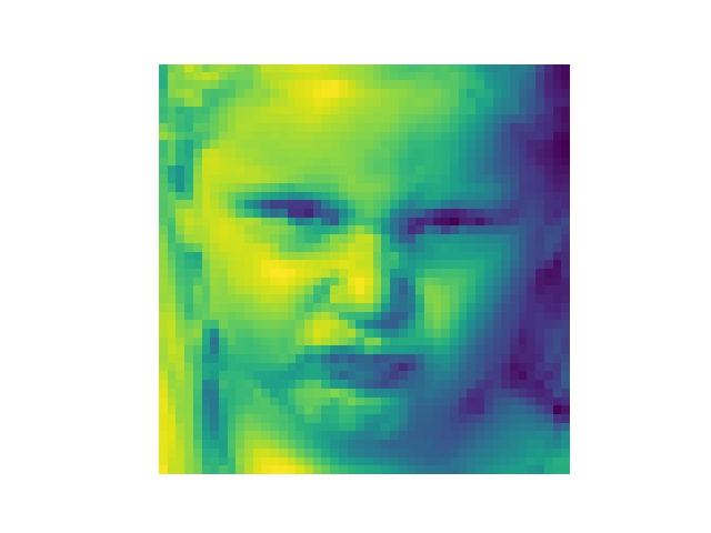
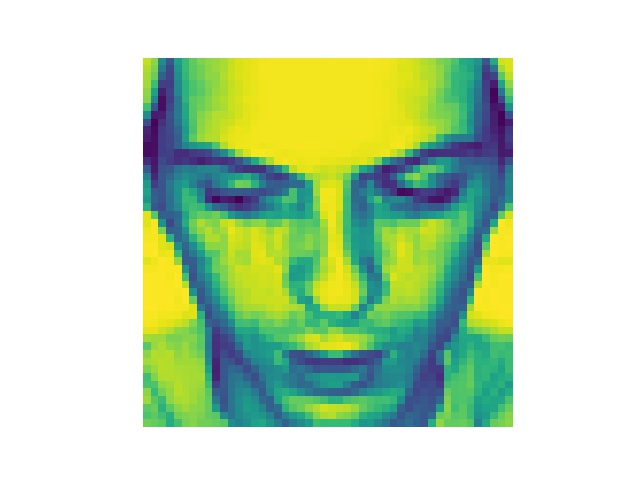
training data前十张图片

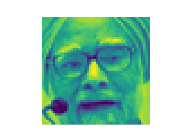
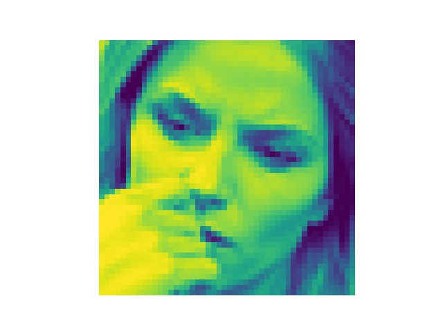

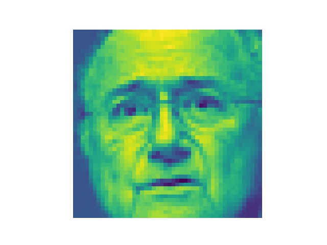
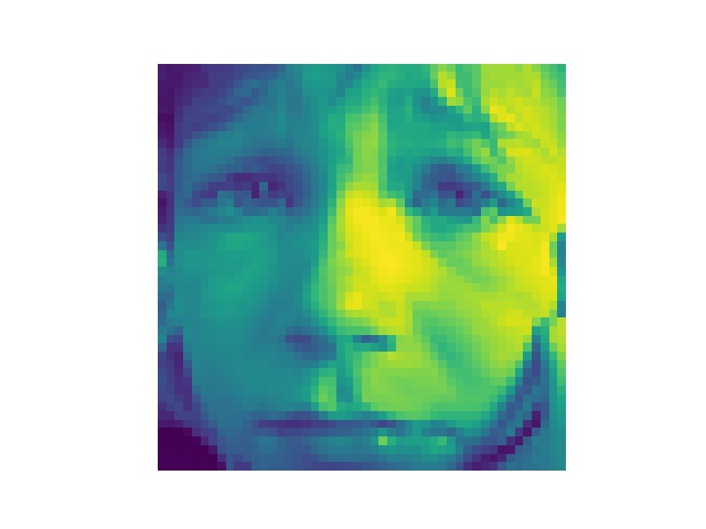

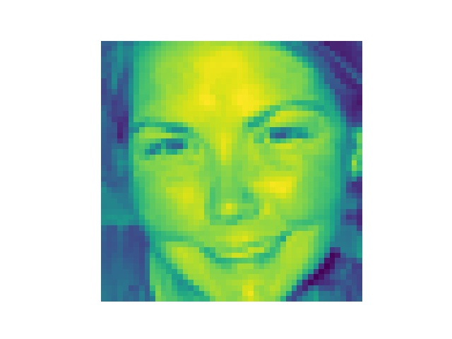

标签分别是
0 Angry 1 Angry 2 Fear 3 Sad 4 Neutral
5 Fear 6 Sad 7 Happy 8 Happy 9 Fear
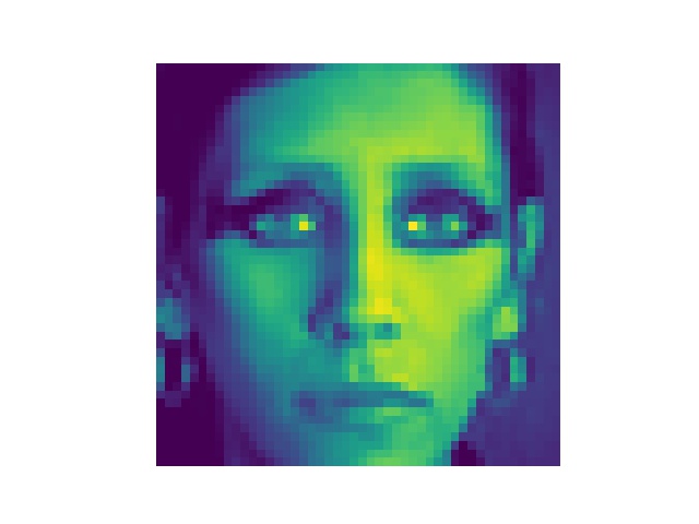
test data前十张照片
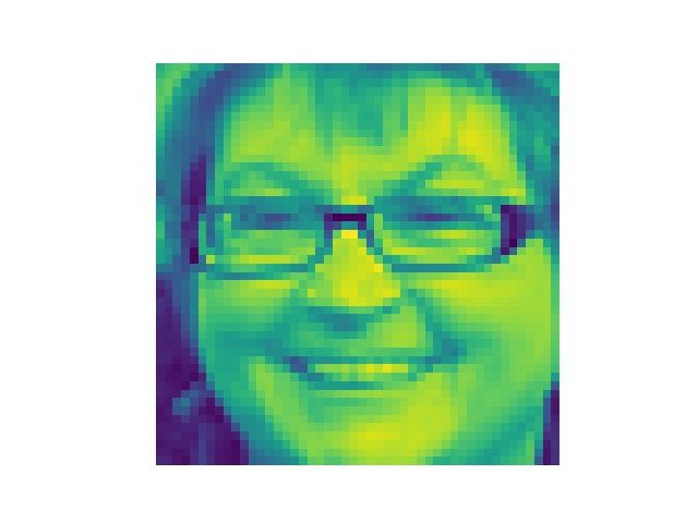


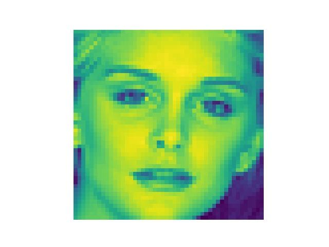
我给出了y_test
0 Happy 1 Happy 2 Happy 3 Happy 4 Neutral
5 Surprise 6 Angry 7 Neutral 8 Fear 9 Neutral
感觉还挺对的啊233
相关代码1
2
3
4
5
6
7
8
9
10
11
12
13
14
15
16
17import matplotlib.pyplot as plt
def show(x_train, y_train, x_val, y_val, x_test):
emo = ['Angry', 'Disgust', 'Fear', 'Happy',
'Sad', 'Surprise', 'Neutral']
for i in range(10):
plt.imshow(x_train[i])
plt.axis('off')
plt.savefig('pic'+str(i)+'.jpg')
plt.show()
print(i, emo[y_train[i]])
for i in range(10):
plt.imshow(x_test[i])
plt.axis('off')
plt.savefig('test_pic'+str(i)+'.jpg')
plt.show()
下面就是有关Model的部分
这是train出最好结果的Model结构print(model.summary())
1 | Layer (type) Output Shape Param # |
第一个卷积层参数print(model.get_layer('conv2d_1').get_weights())
1 | [array([[[[ 1.98697541e-02, 7.08070025e-02, 2.13078111e-02, |
每一块是32个,一共26块,前面是weight,后面是bias吧…
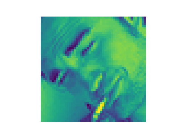
将training data第一张图丢进第一个卷积层中得到的结果

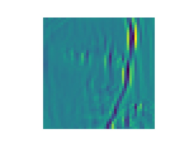

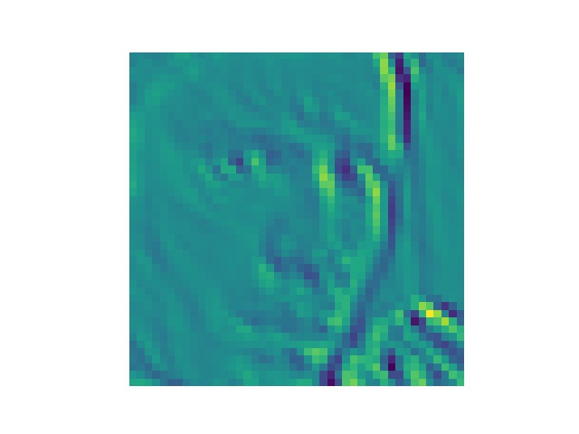
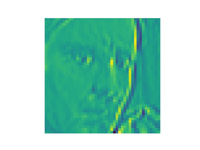

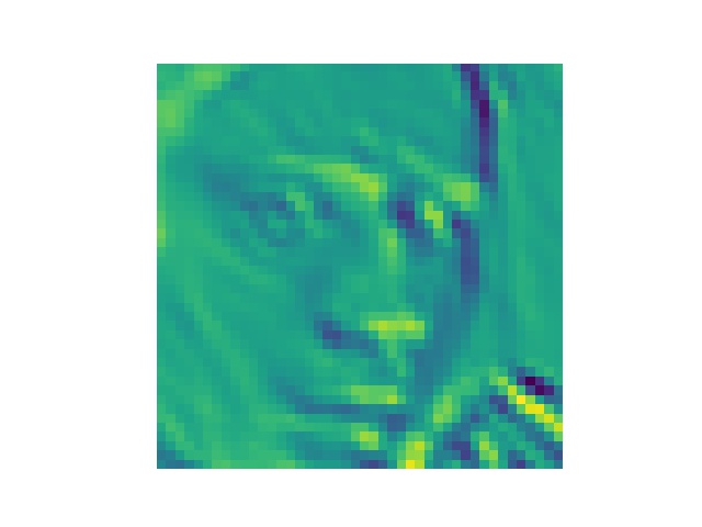
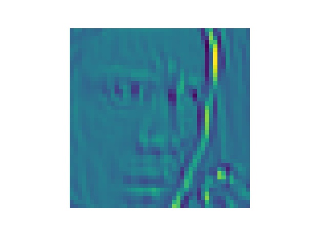
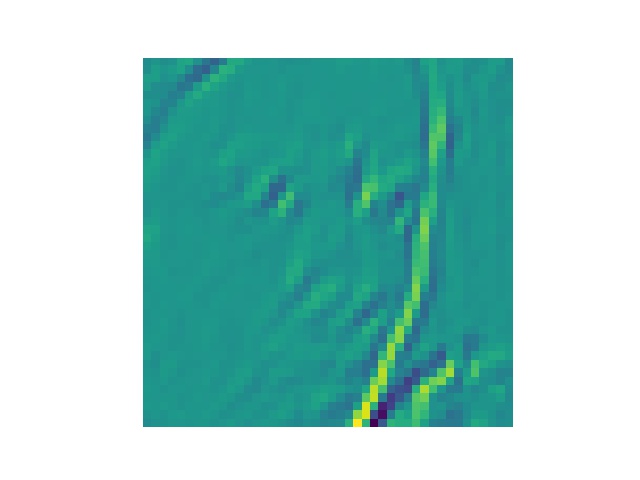

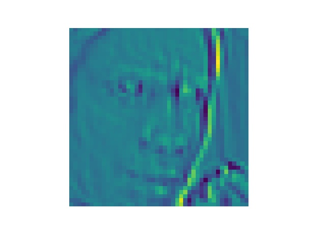
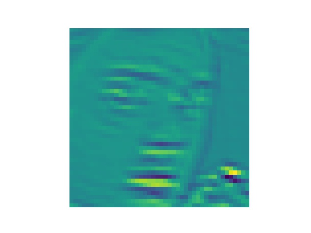

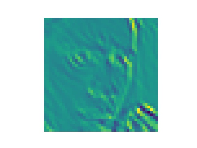
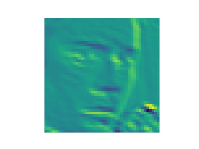
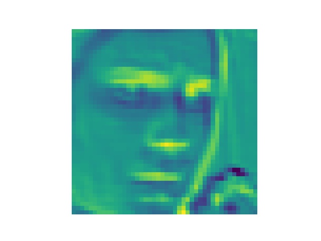


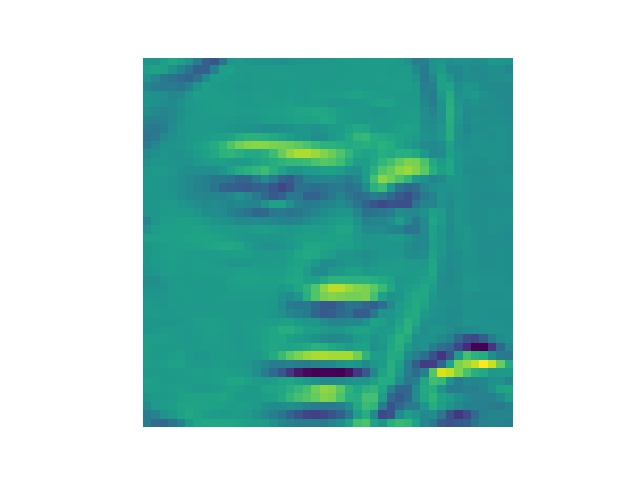
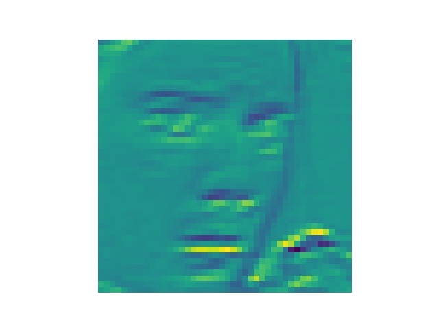

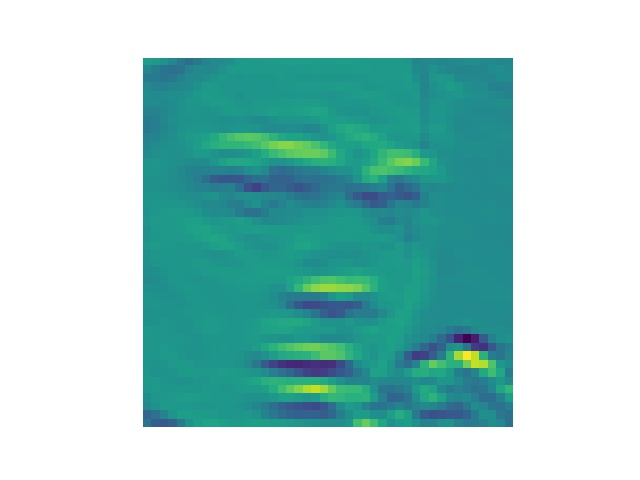
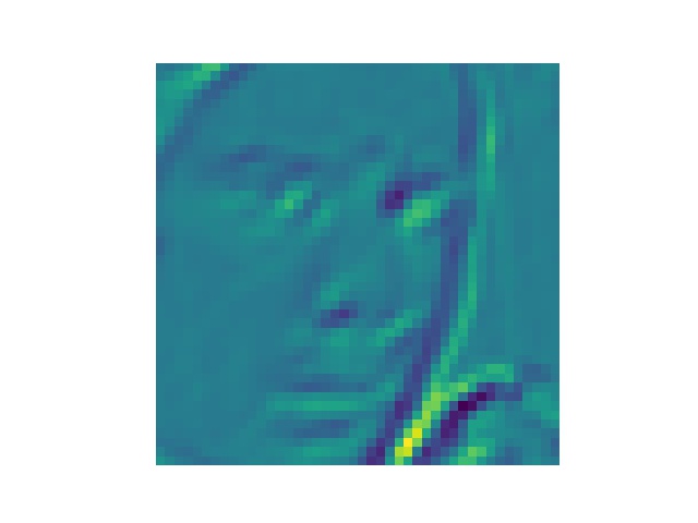
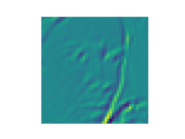
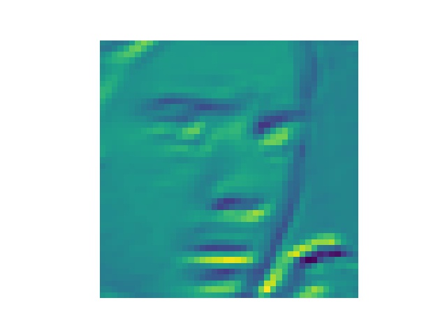
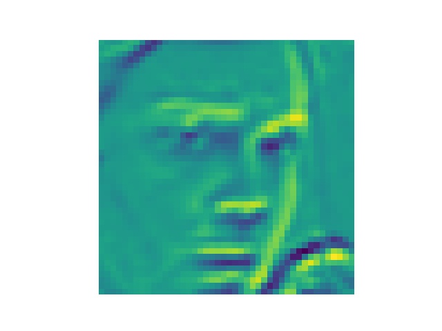
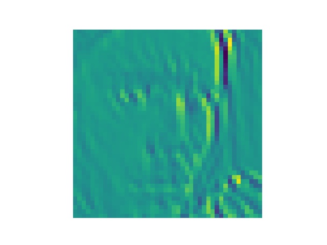
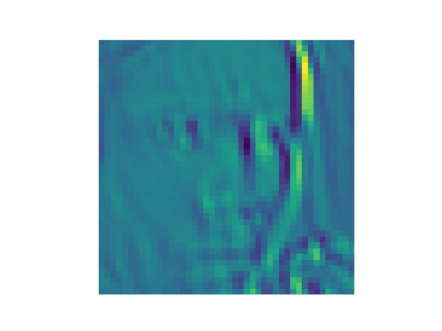


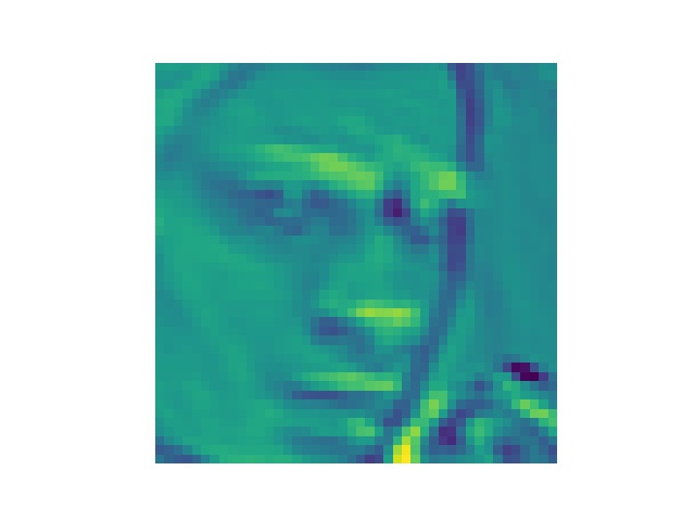
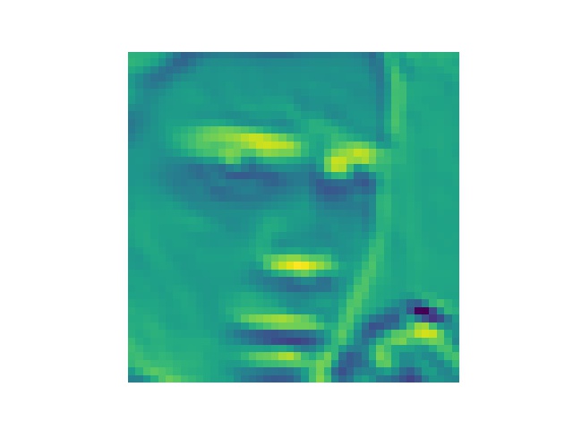

第32张为什么加载不出来?????
最后一张是原图,可以看出来有些感觉就是变成惊讶或者悲伤的样子的,有些特别处理了眉毛,有些特别处理了眼睛的样子吧..
(纯属口胡,我觉得我该好好看看相关论文了
相关代码1
2
3
4
5
6
7
8
9
10
11def show(model, x_train, y_train):
#print(model.get_layer('conv2d_1').get_weights())
layer_model=Model(inputs=model.input,outputs=model.layers[0].output)
t = layer_model.predict(x_train)
print(t, t.shape)
for i in range(32):
plt.imshow(t[0, :, :, i])
plt.axis('off')
plt.savefig('showpic'+str(i)+'.jpg')
plt.show()