机器学习笔记

暑假不定时更新ing…
写好的笔记可能不会立刻同步…可能大部分放英文，小部分中文翻译

Overview & Learning Map

supervised learning

regression
classification
- linear model
- non-linear model
  - deep learning
  - SVM, decision tree, K-NN…
structured learning

semi-supervised learning
transfer learning
unsupervised learning
reinforcement learning
这些根据scenario的不同选择的

The Next Step for Machine Learning

Anomaly Detection (让机器知道”我不知道“)
Explainable AI (为什么知道)
防止 Adversarial Attack
Life-long Learning
Meta-learning / Learn to learn
Few-shot / Zero-shot Learning
增强式学习
Network Compression
如果训练资料和测试资料很不一样

Regression

Step1: Model 模型

首先要有一个Model，也就是一个Function Set，存各种各样的函数。
像$y=b+\sum w_ix_i$这种模型，就是一个Linear Model 线性模型
$x_i$表示attribute of input x，也就是$x$的各种属性feature 特征
$w_i$表示weight权重
$b$表示bias偏差

Step2: Goodness of Function

接下来就是训练模型，选出一个较好的Function
首先要有Training Data，用hat表示正确的数据也就是$\hat{y}$
然后有另一个Function，也就是Loss Function，$L$来评价来估价，例如用平方差估价
$L(f)=L(w,b)=\sum_{n}(\hat{y}^n-(b+w\cdot x^n_{cp}))^2$，得到Estimation Error 估测误差，以下便用这个函数估价

Step3: Best Function

Pick the “Best” Function, $f^{\ast}=arg \min L(f) $ 或 $w^{\ast},b^{\ast}=arg \min L(w,b) $
在这个问题求解的地方
用到了Gradient Descent 梯度下降的方法

Gradient Descent

首先必须是一个可微分的方程，先假设只有一个参数$L(w)$，那我们要求的就是$w^{\ast}=arg\min_{w}L(w)$，步骤如下：
随机选取或稍微优化选取一个初始解$w^{0}$
然后计算$\left . \frac{\text{d}L}{\text{d}w} \right |_ {w=w^{0}}$
显然$\left . \frac{\text{d}L}{\text{d}w} \right |_ {w=w^{0}}$为负，那么右边高损失大，左边低损失小
那么就让$w^{n}=w^{n-1}-\eta \left . \frac{\text{d}L}{\text{d}w} \right |_ {w=w^{n-1}}$
这里$\eta$表示Learning rate，$\eta$越大学习效率越高
然后多次迭代，最后显然是会得到一个Local optimal 局部最优解，也就是导数为零的时候，但不一定是Global optimal 全局最优解。

如果有两个参数$w^{\ast},b^{\ast}=arg \min L(w,b) $，步骤也差不多，求偏微分就是了
$w^{n}=w^{n-1}-\eta \left . \frac{\partial L}{\partial w}\right |_ {w=w^{n-1},b=b^{n-1}},b^{n}=b^{n-1}-\eta \left . \frac{\partial L}{\partial b}\right |_ {w=w^{n-1},b=b^{n-1}}$
那么Gradient就是$\triangledown L=\begin{bmatrix}\frac{\partial L}{\partial w}\\ \frac{\partial L}{\partial b}\end{bmatrix}_ {gradient}$
刚学过偏微分的我还是知道$(-\eta \frac{\partial L}{\partial w},-\eta \frac{\partial L}{\partial b})$的方向，对$L$的微分最大，也是空间的法线方向

在这里没有局部最优解，因为我们定义的函数是convex 凸的，只有全局最优解

Generalization

我们这样可以得到$w,b$，而我们关心的不是训练数据里的损失值，而是Testing Data 测试数据中的数据。

Model Selection

我们想要得到更准确的数据呢，就需要复杂的Model，比如增加三次方，四次方，五次方之类的
A more complex model does not always lead to better performance on testing data. This is Overfitting.
但是复杂的Model在Training Data上的结果很好，但是在Testing Data上的结果较差，这就是Overfitting 过拟合。

Redesign the Model

这时候还会有一个情况，那就是其他隐藏的参数，那就需要重新设计Model
如果是Pokemon的物种，那么就需要if来判断，用$\delta(x_s=x_0)$这个函数来将原函数改写成线性模型，函数值就是里面的等式成立是1不成立就是0

Regularization

就是修改Loss Function
$L=\sum_{n}(\hat{y}^n-(b+\sum w_ix_i))^2+\lambda (w_i)^2$，这里也就是我们希望参数越小越好，这里也是不需要$b$也就是bias的。
如果输入加上一点点变化，我们希望输出不那么参数小也就是输出对输入不那么敏感 sensitive，也就是比较smooth 平滑的。
If some noises corrupt input $x_i$ when testing. A smoother function has less influence.
Training error: larger $\lambda$, considering the training error less.
We prefer smooth function, but don’t be too smooth.

Demo

最后有一个Demo，就是实际操作的时候可能不太好选取Learning Rate也就是$\eta$，用了一个AdaGrad，并对$w,b$分别设置了Learning rate。

Bias and Variance

Review

Error due to “bias” and “variance”.

Estimator

举个栗子，如果要估测$x$的mean 平均值
assume the mean of $x$ is $\mu$
assume the variance of $x$ is $\sigma^2$

那么我们估测平均值$\mu$就随机取$N$个点来计算
$m=\frac{1}{N}\sum_{n}x^n\neq \mu$
$E[m]=E[\frac{1}{N}\sum_{n}x^n]=\frac{1}{N}\sum_{n}E[x^n]=\mu$，$m$的期望就是$\mu$，这个是unbiased的
$Var[m]=\frac{\sigma^2}{N}$，这个Variance depends on the number of samples，如果数量较多那么就会比较集中，如果较少那么就会比较分散了

如果估测variance $\sigma^2$
$m=\frac{1}{N}\sum_{n}x^n\neq \mu,s^2=\frac{1}{N}\sum_{n}(x^n-m)^2$
这里这个$s^2$是biased的，$E[s^2]=\frac{N-1}{N}\sigma^2$

Variance

如果$E[f^{\ast}]=\bar{f}$，那么这个$\bar{f}$和中心店偏移的距离就是bias，而其他$f$和$\bar{f}$分散的距离就是variance
Model 比较简单那么可能获得一个Small Variance的情况，而比较复杂的Model 可能得到一个Large Variance
因为比较简单的Model受数据的影响较小

Bias

$E[f^{\ast}]=\bar{f}$
Bias: If we average all the $f^{\ast}$, is it close to $\hat{f}$
然而一个简单的Model会有比较大的Bias，而比较复杂的Model便有一个小的Bias。

当你的function set的space比较小Model简单，那么它可能不包含target；Model复杂时，function set 的space也变大，就有可能包含target。

我们所得到的Error就是这两个造成的Error的和
如果Error在Bias较小Variance较大的地方就是Overfitting，如果Error在Bias较大Variance较小的地方就是Underfitting 欠拟合

Large Bias

Diagnosis：

If your model cannot even fit the training examples, then you have large bias.
If you can fit the training data, but large error on testing data, then you probably have large variance

For bias, redesign your model:

Add more features as input.
A more complex model.

Large variance

More data
这个可以自己生成许多训练数据
Regularization
这时调整了function space，可能会影响到bias，需要调整weight来取得平衡

Model Selection

There is usually a trade-off between bias and variance.
Select a model that balances two kinds of error to minimize total
Cross Validation
将Training Set分成Training Set和Validation Set，然后用Validation Set来选择Model

如果你把Public Testing Set考虑进去来修改那么就考虑进去了Public Testing Set的bias…

N-fold Cross Validation
分成多份，将其中一份当成Validation Set

Gradient Descent

可以把参数写成向量的形式
那么${\theta}^{\ast}=arg\min_{\theta}L(\theta)$
Gradient:$\triangledown L=\begin{bmatrix}\frac{\partial L(\theta_1)}{\partial \theta_1}\\ \frac{\partial L(\theta_2)}{\partial \theta_2}\end{bmatrix}$
$\theta^{n}=\theta^{n-1}-\eta \triangledown L(\theta^{n-1})$

Tip 1: Tuning your learning rate

Adaptive Learning Rates

Popular & Simple Idea: Reduce the learning rate by some factor every few epochs.
就是说经过几次计算后越来越接近最优解，就要调小Learning Rate，比如$\eta^t=\eta/\sqrt{t+1}$这个压子
Learning rate cannot be one-size-fits-all
Give different parameters different learning rates.

Adagrad

Divide the learning rate of each parameter by the root mean square the its previous derivatives.
Adagrad: $w^{t+1}=w^{t}-\frac{\eta^{t}}{\sigma^{t}}g^{t},\sigma^{t}=\sqrt{\frac{1}{t+1}\sum_{i=0}^{t}(g^{i})^2},\eta^t=\eta/\sqrt{t+1}$
$\sigma^{t}$：root mean square of the previous derivatives of parameter w，就是前面所有的微分的平方的平均值再开根号
约分一下得到$w^{t+1}=w^{t}-\frac{\eta}{\sqrt{\sum_{i=0}^{t}(g^{i})^2}}g^{t}$

Adagrad呢，上面$g^{t}$越大，变化越大，而下面的$\sqrt{\sum_{i=0}^{t}(g^{i})^2}$，会导致$g^{t}$越大，变化越小
Adagrad就是强调一个反差，how suprise it is，下面的考虑的是估计一下二次微分

考虑多个参数时，$g^t$越大，Gradient Descent不一定越大

Tip 2: Stochastic Gradient Descent

Loss函数$L=\sum_{n}\left (\hat{y}^n-(b+\sum w_ix_i^n) \right )^2$
这里要做的就是随机一个$x^n$，$L=\left (\hat{y}^n-(b+\sum w_ix_i^n) \right )^2,\theta^i=\theta^{i-1}-\eta \triangledown L^n(\theta^{i-1})$
有一个Sample就更新一下参数这个样子

Tip 3: Feature Scaling

Make different features have the same scaling.
常见做法：
$R$个向量组$x^i$，For each dimension $i$，都算mean: $m_i$,standard deviation: $\sigma_i$
对第$r$个向量组$x^r$，$x_i^r=\frac{x_i^r-m_i}{\sigma_i}$，这样做完之后呢，所有的mean 会变成0，standard deviation 会变成1

Theory

Taylor Series
理论主要是泰勒展开这个样子，大于等于二次项全部略去，然后相当于在一个圆圈中找一个向量与一次导数组成的向量内积最小，也就是一次导数组成的向量的反方向，再乘上一个常数指到圆圈边界，就得到了Gradient Descent的形式
这也就可以解释Learning Rate设置不对的时候偏差较大的问题

More Limitation of Gradient Descent
会Stuck at Local minimum or saddle point
Very slow at the plateau

Classification: Probabilistic Generative Model

Ideal Alternatives

Function(Model): x->f(x):g(x)>0?class=1:class2
Loss function: $L(f)=\sum_{n}\delta (f(x^n)\neq \hat{y}^n)$, The number of times f get incorrect results on training data
Find the best function: Perceptron, SVN

Generative model

$P(C_1|x)=\frac{P(x|C_1)P(C_1)}{P(x|C_1)P(C_1)+P(x|C_2)P(C_2)}$
$P(x)=P(x|C_1)P(C_1)+P(x|C_2)P(C_2)$

Prior

Assume the points are sampled from a Gaussian distribution.
Find the Gaussion distribution behind them

Gaussian Distribution:
$f_{\mu,\Sigma}(x)=\frac{1}{(2\pi)^{D/2}}\frac{1}{|\Sigma|^{1/2}}\exp\{-\frac{1}{2}(x-\mu)^{T}\Sigma^{-1}(x-\mu)\}$
Input: vector x, output: probability of sampling x
The shape of the function determines by mean $\mu$ and convariance matrix $\Sigma$
这部分有空可以再详细看下

How to find $\mu$ and $\Sigma$ ?

Maximum Likelihood
我们假设这些向量由一个高斯分布generate，要找一个Gussian$(\mu^{\ast},\Sigma^{\ast})$ with maximum likelihood.
$L(\mu,\Sigma)=f_{\mu,\Sigma}(x^1)f_{\mu,\Sigma}(x^2)…f_{\mu,\Sigma}(x^n)$.
$\mu^{\ast},\Sigma^{\ast}=arg\max_{\mu,\Sigma}L(\mu,\Sigma)$.
$\mu^{\ast}=\frac{1}{n}\sum {x^i}(average x),\Sigma^{\ast}=\frac{1}{n}\sum (x^i-\mu^{\ast})(x^i-\mu^{\ast})^{T}$

Modifying Model

公用同一个$\Sigma$，$\Sigma=P(C_1)\Sigma^1+P(C_2)\Sigma^2$，加权平均

Bernoulli distributions

Naive Bayes Classifier

Posterior Probability

$P(C_1|x)=\frac{P(x|C_1)P(C_1)}{P(x|C_1)P(C_1)+P(x|C_2)P(C_2)}=\frac{1}{1+\frac{P(x|C_2)P(C_2)}{P(x|C_1)P(C_1)}}$
Let $z=\ln \frac{P(x|C_1)P(C_1)}{P(x|C_2)P(C_2)}$
$=\frac{1}{1+\exp(-z)}=\sigma(z)$ Sigmoid function

这里$z$是可以化简的
$P(x|C_1)=\frac{1}{(2\pi)^{D/2}}\frac{1}{|\Sigma|^{1/2}}\exp\{-\frac{1}{2}(x-\mu^1)^{T}\Sigma^{-1}(x-\mu^1)\}$.
$P(x|C_2)=\frac{1}{(2\pi)^{D/2}}\frac{1}{|\Sigma|^{1/2}}\exp\{-\frac{1}{2}(x-\mu^2)^{T}\Sigma^{-1}(x-\mu^2)\}$.
$P(C_1)=\frac{N_1}{N_1+N_2},P(C_2)=\frac{N_2}{N_1+N_2}$.

$z=\ln \frac{P(x|C_1)}{P(x|C_2)}+ \ln \frac{P(C_1)}{P(C_2)}=\ln \frac{N_1}{N_2}-\frac{1}{2}[(x-\mu^1)^{T}\Sigma^{-1}(x-\mu^1)-(x-\mu^2)^{T}\Sigma^{-1}(x-\mu^2)]$

把后面的展开$(x-\mu^1)^{T}\Sigma^{-1}(x-\mu^1)=x^{T}\Sigma^{-1}x-x^{T}\Sigma^{-1}\mu^1-(\mu^1)^{T}\Sigma^{-1}x+(\mu^1)^{T}\Sigma^{-1}\mu^1$
中间两项其实是一样的，可以合并，因为右乘一个矩阵和左乘转置矩阵是一样的。
又因为$\Sigma$相同，所以最后可以化成

$z=(\mu^1-\mu^2)^{T}\Sigma^{-1}x-\frac{1}{2}(\mu^1)^{T}\Sigma^{-1}\mu^1+\frac{1}{2}(\mu^2)^{T}\Sigma^{-1}\mu^2+\ln \frac{N_1}{N_2}$

只有第一项包含$x$，后面就是常数，所以可以写成$z=w^{T}\cdot x+b$的形式，要算的就是$\mu^1,\mu^2,\Sigma^{-1}$

Classification: Logistic Regression

我们想要找到一个函数$P(C_1|x)=\sigma(z),z=w\cdot x+b$
当$P(C_1|x)\geqslant 0.5$时输出Class1，反之输出Class2这样子
$f_{w,b}(x)=\sigma(\sum_{i}w_ix_i+b)$ output是0到1之间的数
如果$x^1,x^2$属于Class1，$x^3$属于Class2，$L(w,b)=f_{w,b}(x^1)f_{w,b}(x^2)(1-f_{w,b}(x^3))…$
我们要找$w^{\ast},b^{\ast}=arg\max_{w,b}L(w,b)\Leftrightarrow arg \min_{w,b}-\ln L(w,b)$
为了统一函数，我们给每个设置$\hat{y}$，如果属于Class1，$\hat{y}=1$，否则$\hat{y}=0$
这样对于每一个$-\ln f_{w,b}(x^1)=-[\hat{y}^1\ln f(x^1)+(1-\hat{y}^1)\ln (1-f(x^1))]$
最后我们要minimize的$-\ln L(w,b)=\sum_{n}-[\hat{y}^n\ln f(x^n)+(1-\hat{y}^n)\ln (1-f(x^n))]$
后面这个好像叫做Cross entropy between two Bernoulli distribution，用于评价两个函数有多接近？

最后一步用Gradient Descent来求$w^{\ast},b^{\ast}$就行了
$w_{i+1}=w_{i}-\eta \sum_{n} -(\hat{y}-f_{w,b}(x^n))x_i^n$和Linear regression的式子一样的

Logistic Regression + Square Error ?

主要是求微分以后，离Target最近和最远，微分全都是0

Discriminative v.s. Generative

因为我们假设的不一样，所以Logistics Regression 也就是 Discriminative Model 和 Generative Model找出来的$w$和$b$是不同的
一般来说，Discriminative Model performance会比 Generative Model更好

Benefit of generative model

With the assumption of probability distribution, less training data is needed.
With the assumption of probability distribution, more robust to the noise.
Priors and class-dependent probabilities can be estimated from different sources.

Generative model因为有假设，所以可能会无视一些数据，受数据影响较小，所以可能数据量小时表现会比较好，数据量大的时候就比Discriminative Model 表现较差了

Multi-class Classification

对于每一个Class，都有$w^i,b_i,z_i=w^i\cdot x +b_i$
然后做Softmax，就是强化最大和最小值的差距，然后把概率控制下
$y_i=e^{z_i}/\sum_{n}e^{z_n}$
然后算$y_i$和$\hat{y}_ i$的Cross Entropy $-\sum_{i}\hat{y}_ i\ln y_i$
$\hat{y}$几类就设置成几维，然后自己属于哪一维，那一维就为1，其他为0

Limitation of Logistic Regression

最简单的，比如$(0,0),(1,1)$一类，$(0,1),(1,0)$一类，Logistic Regression就爆炸了

Feature Transformation
就把Logistics Regression接起来用，用几次以后当成转换后的值，在做Logistic Regression。
我们把每一个Logistic Regression叫做一个Neuron，串起来就是Neuron Network 类神经网络，就到了 Deep Learning

先看到这里，我再学一下Python，做一下下作业，不然光看也没啥用…

Deep Learning

Ups and downs of Deep Learning

1958: Perceptron (linear model)
1969: Perceptron has limitation
1980s: Multi-layer perceptron
- Do not have significant difference from DNN today
1986: Backpropagation
- Usually more than 3 hidden layers is not helpful
1989: 1 hidden layer is “good enough”, why deep?
2006: RBM initialization (breakthrough)
2009: GPU
2011: Start to be popular in speech recognition
2012: win ILSVRC image competition

真的是感觉有些不太完善…

Three Step of Deep Learning

跟Machine Learning的三步一样，第一步也就是一个Neural Network

Neural Network: Different connection leads to different network structures.
Network parameter $\theta$ :all the weights and biases in the “neurons”.

Fully Connect Feedforward Network

如果我们知道所有的weights和bisaes，那么这其实就是一个function
如果只知道structure不知道这些，那么就是一个function set

一共分成三层
input layer - hidden layers - output layer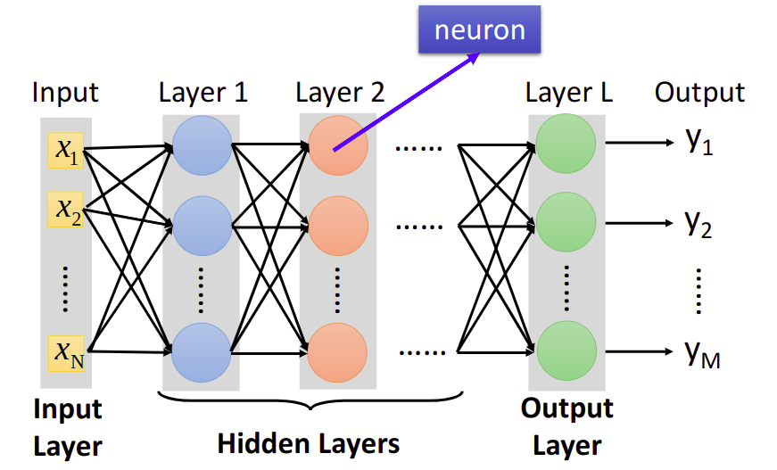

Deep = Many hidden layers

Matrix Operation: 其实就是input vector 来进行matrix operation （每一层集合所有的weights 和 biases，每一层最后有一个activation function），最后得到output vector
矩阵运算可以GPU加速

feature extractor replacing feature engineering

Backpropagation

在Neutral Network里面做Gradient Descent有很多参数，那么怎么求Gradient呢
就是用Backpropagation

Chain Rule

就是链式求导法则
要求$\frac{\partial L}{\partial w}$, $L=\sum C^n$，$C^n$就是评价$y$和$\hat{y}$之间距离的函数
那么$\frac{\partial L}{\partial w}=\sum \frac{\partial C^n}{\partial w}$
而$\frac{\partial C}{\partial w}=\frac{\partial z}{\partial w}\frac{\partial C}{\partial z}$

Forward pass: Compute $\frac{\partial z}{\partial w}$ for all parameters.
Backward pass: Compute $\frac{\partial C}{\partial z}$ for all activation function inputs z, Compute $\frac{\partial C}{\partial z}$ from the output layer.
有一些细节，就是从后往前算，需要乘上weight然后经过op-amp乘上一个常数得到
其实就是建一个反向Neural Network来计算，output变成input

Keras

Interface of TensorFlow or Theano
Easy to learn and use(still have some flexibility)

安装 & 使用：https://keras.io/

1 2	sudo pip install tensorflow sudo pip install keras

但是遇到了一个问题…

    Complete output from command python setup.py egg_info:
    Traceback (most recent call last):
      File "<string>", line 1, in <module>
      File "/tmp/pip-build-aAiWd2/scipy/setup.py", line 31, in <module>
        raise RuntimeError("Python version >= 3.5 required.")
    RuntimeError: Python version >= 3.5 required.
    
    ----------------------------------------
Command "python setup.py egg_info" failed with error code 1 in /tmp/pip-build-aAiWd2/scipy/

我Python明明是3.7，为啥就不行了呢，后来我想起来我装了Anaconda以后都是在虚拟环境中，所以，不加sudo就能安装了

Mini-batch

one epoch

Randomly initialize network parameters
Pick the 1st batch, Update parameters once
Pick the 2nd batch, Update parameters once
Until all mini-batches have been picked

Repeat the above process

设置这个可以利用GPU加速

Tip for Deep Learning

Recipe of Deep Learning

两个问题：一个是在Training Data上performance不好，一个是在Testing Data上performance不好

Bad Results on Training Data

两种方法

New activation function
Adaptive Learning Rate

有一种情况，靠近input layer的地方微分值很小，Learn very slow，Almost random；靠近ouput layer的地方微分值较大，Learn very fast，Almost converge。这件事发生的原因是使用sigmoid function，一个很大的$\Delta$经过sigmoid function以后是会变小的，而且影响也会越来越小。
解决的方法呢

Rectified Linear Unit(ReLU)

$\sigma(z)=\left\{\begin{matrix} a=z, && z\geqslant 0\\ a=0, && z<0 \end{matrix}\right.$

Reason:

Fast to compute
Biological reason
Infinite sigmoid with different biases
can handle vanishing gradient
当它去掉output为0的点以后，得到一个Thinner linear network，不再有smaller gradients，不会递减了
ReLU variant
Leaky ReLU:$\sigma(z)=\left\{\begin{matrix}a=z, && z\geqslant 0\\ a=0.01z, && z<0\end{matrix}\right.$
Parametric ReLU: $\sigma(z)=\left\{\begin{matrix}a=z, && z\geqslant 0\\ a=\alpha z, && z<0\end{matrix}\right., \alpha also learned by gradient descent$

Maxout

ReLU is a special class of Maxout
Learnable activation function.
就是把几个neurons划到同一个组，选一个最大的当做output作为下一层的input
Activation function in maxout network can be any piecewise linear convex function
How many pieces depending on how many elements in a group.

Maxout - Training
就是train一个thin and linear network，差不多就是把选中的部分提出来train
Different thin and linear network for different examples.

下面都是第二种方法

RMSProp

Adagrad是Use first derivative to estimate second derivative
RMSProp是这样计算的 Root Mean Square of the gradients with previous gradients being decayed
$w^{1}\leftarrow w^{0}-\frac{\eta}{\sigma^{0}}g^{0}, \sigma^{0}=g^{0}$
$w^{2}\leftarrow w^{1}-\frac{\eta}{\sigma^{1}}g^{1}, \sigma^{1}=\sqrt{\alpha (\sigma^{0})^2+(1-\alpha)(g^{1})^{2}}$
$w^{n+1}\leftarrow w^{n}-\frac{\eta}{\sigma^{n}}g^{n}, \sigma^{n}=\sqrt{\alpha (\sigma^{n-1})^2+(1-\alpha)(g^{n})^{2}}$

Momentum

Movement: movement of last step minus gradient at present

Step:
Start at point $\theta^{0}$
Movement $v^{0}=0$
Compute gradient at $\theta^{0}$
Movement $v^{1}=\lambda v^{0}-\eta \triangledown L(\theta^{0})$
Move to $\theta^{1}=\theta^{0}+v^{1}$
Compute gradient at $\theta^{1}$
Movement $v^{2}=\lambda v^{1}-\eta \triangledown L(\theta^{1})$
Move to $\theta^{2}=\theta^{1}+v^{2}$

Movement not just based on gradient, but previous movement.
$v^{i}$ is actually the weighted sum of all the previous gradient: $\triangledown L(\theta^{0}),\triangledown L(\theta^{1}),…,\triangledown L(\theta^{i-1})$

Adam: RMSProp + Momentum

这里字太多了…我就截图了
算法：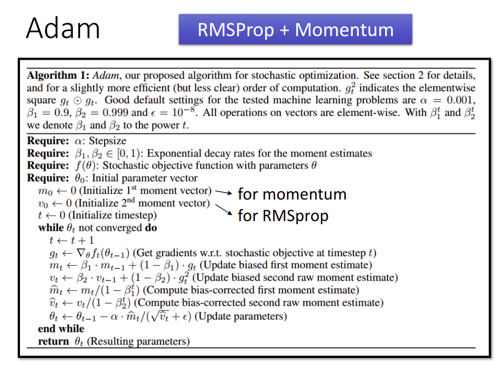

Bad Results on Testing Data

Early Stopping

用Validation set模拟Testing set选一个Validation set上loss较小的点停下来，而不是一直Train下去

Regularization

New loss function to be minimized

Find a set of weight not only minimizing original cost but also close to zero
$L’(\theta)=L(\theta)+\lambda \frac {1}{2} \begin{Vmatrix}\theta\end{Vmatrix}_ {2},\theta=\{w_1,w_2,…\},\begin{Vmatrix}\theta\end{Vmatrix}_ {2}=(w_1)^2+(w_2)^2+…$.
就是找一个尽量平滑的函数嘛，后面那个Regularization term就是使函数平滑
这里是$\theta$的L2 norm，也叫作L2 regularization
做Regularization一般不会考虑biases，因为只是平滑函数而已

微分一下$Gradient:\frac{\partial L’}{\partial w}=\frac{\partial L}{\partial w}+\lambda w$.
$Update: w^{t+1}=w^{t}-\eta \frac{\partial L’}{\partial w}=(1-\eta \lambda)w^{t}-\eta \frac{\partial L}{\partial w}$.
会让参数越来越大接近0，每次都让weight小一点，叫做Weight Decay

同样的L1 Regularization
$L’(\theta)=L(\theta)+\lambda \frac {1}{2} \begin{Vmatrix}\theta\end{Vmatrix}_ {1},\theta=\{w_1,w_2,…\},\begin{Vmatrix}\theta\end{Vmatrix}_ {1}=|w_1|+|w_2|+…$.
$Gradient:\frac{\partial L’}{\partial w}=\frac{\partial L}{\partial w}+\lambda sgn(w)$.
$Update: w^{t+1}=w^{t}-\eta \frac{\partial L’}{\partial w}=w^{t}-\eta \frac{\partial L}{\partial w}-\eta \lambda sgn(w^{t})$.
L1每次都减去一个固定的值

Dropout

Each time before updating the parameters.
Each neuron has $p\%$ to dropout, the structure of the network is changed.
Using the new network for training.
For each mini-batch, we resample the dropout neurons.

Testing
No dropout
If the dropout rate at training is $p\%$, all the weights times $1-p\%$.
Assume that the dropout rate is $50\%$.
If a weight $w=1$ by training, set $w=0.5$ for testing.

Dropout is a kind of ensemble.
Using one mini-batch to train one network.
Some parameters in the network are shared.

最后这个操作呢，差不多就是假如有$m$个neuron，然后我们train的是$2^m$个Network，然后最后把他们平均起来，如果activation function是线性的话，与平均值是相等的，但如果不是Linear的，两个值呢也是约等的这个样子…
所以Dropout在Linear的activation function上performance是比较好的，比如ReLU和Maxout

这节课好长啊…今天明天再看看Demo做一下hw2好了

Demo

这是Demo1和Demo2的合集，不同情况下修改不同的函数和结构之类的

import numpy as np
from keras.models import Sequential
from keras.layers.core import Dense, Dropout, Activation
from keras.layers import Conv2D, MaxPooling2D, Flatten
from keras.optimizers import SGD, Adam
from keras.utils import np_utils
from keras.datasets import mnist

def load_data():
    (x_train, y_train), (x_test, y_test) = mnist.load_data()
    number = 10000
    x_train = x_train[0:number]
    y_train = y_train[0:number]
    x_train = x_train.reshape(number, 28*28)
    x_test = x_test.reshape(x_test.shape[0], 28*28)
    x_train = x_train.astype('float32')
    x_test = x_test.astype('float32')
    
    y_train = np_utils.to_categorical(y_train, 10)
    y_test = np_utils.to_categorical(y_test, 10)
    x_train = x_train
    x_test = x_test
    x_train = x_train / 255
    x_test = x_test / 255
    x_test = np.random.normal(x_test)
    return (x_train, y_train), (x_test, y_test)

(x_train, y_train), (x_test, y_test) = load_data()

model = Sequential()
#model.add(Dense(input_dim=28*28, units=666, activation='sigmoid'))
model.add(Dense(input_dim=28*28, units=666, activation='relu'))
model.add(Dropout(0.7))
#model.add(Dense(units=666, activation='sigmoid'))
#model.add(Dense(units=667, activation='sigmoid'))
model.add(Dense(units=666, activation='relu'))
model.add(Dropout(0.7))
model.add(Dense(units=667, activation='relu'))
model.add(Dropout(0.7))
#for i in range(10):
#    model.add(Dense(units=666, activation='relu'))
model.add(Dense(units=10, activation='softmax'))

#model.compile(loss='mse', optimizer=SGD(lr=0.1), metrics=['accuracy'])
#model.compile(loss='categorical_crossentropy', optimizer=SGD(lr=0.1), metrics=['accuracy'])
model.compile(loss='categorical_crossentropy', optimizer='adam', metrics=['accuracy'])
model.fit(x_train, y_train, batch_size=100, epochs=20)


result = model.evaluate(x_train, y_train, batch_size=10000)
print('\nTrain Acc:', result[1])

result = model.evaluate(x_test, y_test, batch_size=10000)
print('\nTest Acc:', result[1])

Convolutional Neural Network

Why CNN for image

Some patterns are much smaller that the whole image
A neuron does not have to see the whole image to discover the pattern, Connecting to small region with less parameters.
就是一个Nerual不需要看到整个图，只需要连接某一部分就可以了，这样可以减去很多参数,fully connected network需要的参数就太多了

The same patterns appear in different regions

Subsampling the pixels will not change the object.

The whole CNN

repeat : convolution - max pooling
then flatten - fully connected feedforward network

之前已经观察到的Property

Some patterns are much smaller that the whole image.(Convolution)
The same patterns appear in different regions.(Convolution)
Subsampling the pixels will not change the object.(Max Pooling)

CNN - Convolution

每次移动距离stride，每次和filter做内积
Do the same process for every filter
最后得到Feature Map

CNN - Colorful image

Filter 增加一个RGB维度

CNN v.s. Fully connected network

Less parameters，减去一些连接的weights
Even less parameters，shared weights

CNN - Max Pooling

把filter后得到的分组，选最大或选mean都可以，这就把图片缩小了
经过一次Convolution和Max Pooling得到一个新的image，Smaller than the original image,New image but smaller.

Each filter is a channel.
The number of the channel is the number of filters.

Flatten

把Feature Map拉直，然后丢到Fully Connected Network就ok了

CNN in Keras

Only modified the network structure and input format(vector -> 3-D tensor)

Convolution Layer

1	model.add(Convolution2D(25, 3, 3, input_shape=(1, 28, 28))) # 25个33的filter input是1维黑白2828的图片

MaxPooling

1	model.add(MaxPooling2D((2, 2))) # 2*2的featuremap选最大的

Flatten + Fully connected layer

model.add(Flatten())

model.add(Dense(output_dim = 100))
model.add(Activation('relu'))
model.add(Dense(output_dim = 10))
model.add(Activation('softmax'))

What does CNN learn?

Degree of the activation of the k-th filter: $a^k=\sum_{i} \sum_{j} a^{k}_ {ij}$
找一个input$x^{\ast}$,$x^{\ast}=arg \max_x a^k$(gradient ascent)

Find an image maximizing the output of neuron :$x^{\ast}=arg \max_{x} a^{j}$
Each figure corresponds to a neuron

$x^{\ast}=arg \max_{x} y^{i}$
如果是做数字辨识会发现找到最Activation的$x^{\ast}$其实并不是数字
有一个视频https://www.youtube.com/watch?v=M2IebCN9Ht4

做一个限制 L1 regularization
$x^{\ast} = arg \max_{x} (y^{i}-\sum_{i,j}|x_{ij}|)$

Deep Dream
CNN exaggerates what it sees

Deep Style
Given a photo, make its style like famous painting

output 也就是 content像原相片，style也就是filter之间的correlation像风格相片

有很多关于CNN的应用，只需要满足图片的特征就可以了，也就是前面提到的3个property

Demo

这里应该有Demo的…然而视频中莫有

Why Deep Learning ?

相同参数下，越Deep其实performance会变好

Modularization

不同的function可以调用共同的subfunction

Each basic classifier can have sufficient training example
如果要分4类，长发男，长发女，短发男，短发女，但是长发男的数据很少
这样的情况下，不如用两个basic classifer，分长发短发，男女，这样每类的数据都是足够的
Sharing by the following classifiers as module
然后再用4个classifier来分出来，只需要比较少的data就可以了

所以Network的结构
The most basic classifiers
Use 1st layer as module to build classifiers
Use 2nd layer as module…

The modularization is automatically learned from data.
所以Deep Learning需要比较少的Training data？

Universality Theorem

Any continuous function f
can be realized by a network with one hidden layer(given enough hidden neurons)
Yes, shallow network can represent any function.
However, using deep structure is more effective.

End-to-end Learning

只知道input 和 output
What each function should do is learned automatically

所以最后的结论
Do deep nets really need to be deep ? Yes !

Semi-supervised Learning

Introduction

Supervised learning:$\{(x^r,\hat{y}^r)\}^{R}_ {r=1}$

E.g. $x^r$:image, $\hat{y}^{r}$:class labels

Semi-supervised leaning: $\{(x^r,\hat{y}^r)^{R}_ {r=1}\}, \{x^u\}^{R+U}_ {u=R}$

A set of unlabeled data, usually $U>>R$
Transductive learning: unlabeled data is the testing data
Inductive learning: unlabeled data is not the testing data

Why semi-supervised learning

Collecting data is easy, but collecting “labelled” data is expensive
We do semi-supervised learning in our lives

Why semi-supervised learning helps?

The distribution of the unlabeled data tell us something.
就是这些input的分布会影响结果的判断
Usually with some assumptions 通常伴随着一些假设

Semi-supervised Learning for Generative Model

Supervised Generative Model
Given labelled training examples $x^r\in C_1,C_2$

looking for most likely prior probability $P(C_i)$ and class-dependent probability $P(x|C_i)$
$P(x|C_i)$ is a Gaussian parameterized by $\mu^i$ and $\Sigma$

Semi-supervised Generative Model

Initialization:$\theta = \{P(C_1),P(C_2),\mu^{1},\mu^{2},\Sigma\}$
Step1(E): compute the posterior probability of unlabeled data $P_{\theta}(C_1|x^{u})$, Depending on model $\theta$
Step2(M): update model
$P(C_1)=\frac{N_1+\Sigma_{x^u}P(C_1|x^u)}{N}$.
$N$: total number of examples
$N_1$: number of examples belonging to $C_1$
$\mu^{1}=\frac{1}{N_1}\sum_{x^r\in C_1}x^r+\frac{1}{\sum_{x^u}P(C_1|x^u)}\sum_{x^u}P(C_1|x^u)x^u$
Back to step1

The algorithm converges eventually, but the initialization influences the results.

Why?

Maximum likelihood with labelled data(Closed-form solution)
$\log L(\theta)=\sum_{x^r}\log P_{\theta}(x^r,\hat{y}^r), P_{\theta}(x^r,\hat{y}^r)=P_{\theta}(x^r|\hat{y}^r)P(\hat{y}^r)$.
Maximum likelihood with labelled + unlabeled data(Solved iteratively)
$\log L(\theta)=\sum_{x^r}\log P_{\theta}(x^r,\hat{y}^r)+\sum_{x^u}\log P(\theta)(x^u), P_{\theta}(x^u)=P_{\theta}(x^u|C_1)P(C_1)+P_{\theta}(x^u|C_2)P(C_2)$, $x^u$ can come from either $C_1,C_2$.

Semi-supervised Learning - Low-density Separation

Self-training

Given: labelled data set = $\{(x^r,\hat{y}^r)\}^{R}_ {r=1}$, unlabeled data set = $\{x^u\}^{R+U}_ {u=l}$
Repeat:

Train model $f^{\ast}$ from labelled data set.(Independent to the model)
Apply $f^{\ast}$ to the unlabeled data set
- Obtain $\{x^u,y^u\}^{R+U}_ {u=l}$(Pseudo-label)
Remove a set of data from unlabeled data set, and add them into the labeled data set
How to choose the data set remains open
You can also provide a weight to each data.

Similar to semi-supervised learning for generative model
Hard label v.s. Soft lable
neural network的时候一定是用Hard label

Entropy-based Regularization

Entropy of $y^u$: Evaluate how concentrate the distribution $y^u$ is $E(y^u)=-\sum_{m}y^{u}_ {m}\ln (y^{u}_ {m})$, $m$: number of class. As small as possible.
$L=\sum_{x^r}C(y^r,y^r)+\lambda \sum_{x^u}E(y^u)$ 可微分，用Gradient Descent minimize，后面的可以让他不Overfitted

Semi-supervosed Learning Smoothness Assumption

近朱者赤，近墨者黑“You are knownby the companyyoukeep”

Assumption: “similar” $x$ has the same $\hat{y}$
More precisely:
- x is not uniform.
- If $x^1$ and $x^2$ are close in a high density region,$\hat{y}^1$ and $\hat{y}^2$ are the same.
  connected by a high density path

Cluster and then label
Using all the data to learn a classifier as usual

Graph-based Approach
Represented the data points as a graph
Graph representation is nature sometimes.

定性使用
Graph-based Approach - Graph Construction

Define the similarity $s(x^i,x^j)$ between $x^i$ and $x^j$
Add edge:
- K Nearest Neighbor
- e-Neighborhood
Edge weight is proportional to $s(x^i,x^j)$

Gaussion Radial Basis Function
$s(x^i,x^j)=\exp (-\gamma || x^i-x^i ||^2)$

存在的问题
The labelled data influence their neighbors.
Propagate through the graph

定量使用

Define the smoothness of the labels on the graph
$S=\frac{1}{2}\sum_{i,j}w_{i,j}(y^i-y^j)^2$ For all data(no matter labelled or not)
$\mathbf{y}$: (R+U)-dim vector.
$\mathbf{y}=[\cdots y^i \cdots y^j \cdots]^{T}$.
$L$:(R+U) x (R+U) matrix (Graph Laplacian).
$L = D - W$, $W$就是边权建出的图，$D$就是$W$每行的值求和放在$(i,i)$的位置
Then $S=\mathbf{y}^{T}L\mathbf{y}$,$y$ depenting on network parameters
原来Loss Function $L=\sum_{x^r}C(y^r,\hat{y}^r)+\lambda S$, As a regularization term

Semi-supervised Learning - Better Representation

去蕪存菁，化繁為簡

Find the latent factors behind the obvservation.
The latent factors (usually simpler) are better representations.

Unsupervised Learning - Linear Methods

Unsupercised Learning

两类

Clustering & Dimension Reduction(化繁为简)
only having function input.
Generation(无中生有)
only having function output.

这节课主要是Linear 的 Dimension Reduction

Clustering

K-means

Clustering $X=\{x^1, \cdots, x^n, \cdots, x^{N}\}$ into K clusters
Initalize cluster center $c^i, i=1,2,\cdots, K$(K random $x^n$ from X)
Repeat
For all $x^n$ in X: $b^n_i=\left\{\begin{matrix}1 &x^n\text{ is most “close” to }c^i \\ 0 &Otherwise \end{matrix}\right.$
Updating all $c^i$: $c^i=\sum_{x^n}b^n_ix^n/\sum_{x^n}b^n_i$

Hierarchical Agglomerative Clustering(HAC)

Step1: build a tree
建树过程是这样的，$n$个data，选两个最像的做平均连起来变成1个data，这样就有$n-1$个data，继续做下去就可以建一棵树
Step2: pick a threshold
在树上切一刀可以决定分成多少个Cluster

Distributed Representation

Clustering: an object must belong to one cluster
Distributed representation: 用一个vector每一维表示一个attribute
这个将一个object用Distribution representation表示，从高维空间变到低维空间，就是Dimension Reduction.

Dimension Reduction

找一个Function，输入一个高维的vector得到一个低微的vector

Feature selection：把没用的Dimension去掉
Principle component analysis(PCA): $z=Wx$

Principle component analysis(PCA)

Principle component analysis(PCA)主成分分析
$z=Wx$
对于$z$每一维，都是$z_i=w^i \cdot x$
$var(z_i)=\sum_{z_i}(z_i-\bar{z_i})^2, ||w^i||_ 2=1$
$z_i$的variance越大越好
然后$w^i$要两两垂直
$W=\begin{bmatrix}(w^1)^{T} \\ (w^2)^{T} \\ \vdots \end{bmatrix}$.
$W$就是个 Orthogonal matrix 正交矩阵

Lagrange multiplier
$z_1=w^1\cdot x$
$\bar{z_1}=\sum z_1=\sum w^1\cdot x = w^1\sum x=w^1 \cdot x$.
$var(z_1)=\sum_{z_1}(z_1-\bar{z_1})^2=\sum_{x}(w^1\cdot x-w^1\cdot \bar{x})^2=\sum (w^1\cdot (x-\bar{x}))^2$.
$\because (a\cdot b)^2=(a^{T}b)^2=a^{T}ba^{T}b=a^{T}b(a^{T}b)^{T}=a^{T}bb^{T}a$.
$\therefore var(z_1)=\sum (w^1)^{T}(x-\bar{x})(x-\bar{x})^{T}w^1=(w^1)^{T}\sum (x-\bar{x})(x-\bar{x})^{T} w^1=(w^1)^{T}Cov(x)w^1$.
$Cov(x)$是$x$的covariance matrix
Let $S=Cov(x)$, Symmetric, positive-semidefinite,(non-negative eigenvalues)
Find $w^1$ maximizing $(w^1)^{T}Sw^1$.
Constraint: $||w^1||_ 2=(w^1)^{T}w^1=1$
Using Largrange multiplier
$g(w^1)=(w^1)^{T}Sw^1-\alpha ((w^1)^{T}w^1-1)$.
让$\partial g(w^1)/\partial w^1_1 =0,\partial g(w^1)/\partial w^1_2 =0,…$.
然后就得到解$Sw^1-\alpha w^1=0$，即$Sw^1=\alpha w^1$，$w^1$就是$S$的eigenvector 特征向量
$(w^1)^{T}Sw^1=\alpha (w^1)^{T}w^1=\alpha$ Choose the maximum one.

结论：$w^1$ is the eigenvector of the convariance matrix $S$, Corresponding to the largest eigenvalue $\lambda$

Find $w^2$ maximizing $(w^2)^{T}Sw^2$, $(w^2)^{T}w^2=1,(w^2)^{T}w^1=0$.
$g(w^2)=(w^2)^{T}Sw^2-\alpha ((w^2)^{T}w^2-1)-\beta((w^2)^{T}w^1-0)$.
让$\partial g(w^2)/\partial w^2_1 =0,\partial g(w^2)/\partial w^2_2 =0,…$.
$Sw^2-\alpha w^2 - \beta w^1=0$
$(w^2)^{T}Sw^2-\alpha ((w^2)^{T}w^2-1)-\beta((w^2)^{T}w^1-0)=0$.
$((w^1)^{T}Sw^2)^{T}=(w^2)^{T}S^{T}w^1=(w^2)^{T}Sw^1=\lambda_1(w^2)^{T}w^1=0$.
所以$\beta=0: Sw^2-\alpha w^2=0, Sw^2=\alpha w^2$

结论：$w^2$ is the eigenvector of the convariance matrix $S$. Corresponding to the 2nd largest eigenvalue $\lambda_2$.

PCA - decorrelation
$z=Wx,Cov(z)=D$ $Cov(z)$是一个Diagonal matrix
$Cov(z)=\sum(z-\bar{z})(z-\bar{z})^{T}=WSW^{T}, S=Cov(x)$
$=WS[w^1 \cdots w^K]=W[Sw^1 \cdots Sw^K]=W[\lambda_1w^1 \cdots \lambda_Kw^K]=[\lambda_1Ww^2 \cdots \lambda_KWw^zk]=[\lambda_1e_1 \cdots \lambda_Ke_K]$, $e_K$是第$K$维是1其他是0

PCA - Another Point of View

Basic Component: 就是一些基本的组成，每一个都是一个vector, $u^K$
$x\approx c_1u^1+c_2u^2+\cdots + c_Ku^K+\bar{x}$
所以可以用$\begin{bmatrix}c_1\\ c_2\\ \vdots\\ c_K\end{bmatrix}$ represent a image $x$.

$x-\bar{x}\approx c_1u^1+c_2u^2+\cdots + c_Ku^K=\hat{x}$.
Reconstruction error: $||(x-\bar{x})-\hat{x}||_ 2$.
Find $\{u^1,\cdots, u^K\}$ minimizing the error.

$L=\min _ {\{u^1,\cdots ,u^K\}}\sum \left \| (x-\bar{x})-(\sum_{k=1}^{K}c_ku^k) \right \| _ 2$

PCA求得$w^1,\cdots, w^K$其实就是$u^1,\cdots, u^K$，证明好像是线代相关SVD…感觉我们学的线代内容好基础…看不太懂233

PCA looks like a neural network with one hidden layer(linear activation function). Autoencoder
$\hat{x}=\sum_{k=1}^{K}c_kw^k=x-\bar{x}$.
To minimize reconstruction error: $c_k=(x-\bar{x})\cdot w^k$.
可以用一个neural network表示
It can be deep. Deep autoencoder.

Weakness of PCA

Unsupervised
Linear

LDA = linear discriminant analysis，是supervised

What happens to PCA?

PCA involves adding up and subtracting some components(images)

Then the components may not be “parts of digits”
Non-negative matrix factiorization(NMF)
Forcing $a_1,a_2,…$ be non-negative
- adaitive combination
Forcing $w^1,w^2,…$ be non-negative
- More like “parts of digits”

Matrix Factorization

Minimizing $L=\sum(r^i\cdot r^j-n_{ij})^2$
Find $r^i,r^j$ by Gradient Descent.

More about Mareix Factorization

Considering the induvial characteristics
$r^A\cdot r^1\approx 5\rightarrow r^A\cdot b_A+b_1\approx 5$.
$b_A$: otakus A likes to by figures.
$b_1$: how popular character 1 is.
加了另外两个特征
Minimizing $L=\sum_{(i,j)}(r^i\cdot r^j + b_i + b_j -n_{ij})^2$.
Find $r^i,r^j,b_i,b_j$ by gradient descent(can add regularization)

Ref: Matrix Factorization Techniques for Recommender Systems.

Matrix Factorization for Topic analysis
在这方面的应用的方法叫做 Latent semantic analysis(LSA)

Unsupervised Learning: Word Embedding

Word Embedding

Machine learn the meaning of words from reading a lot of documents without supervision.
Genarating Word Vector is unsupervised.

A word can be understood by its context, You shall know a word by the company it keeps.

How to exploit the context

Count based

If two words $w_i$ and $w_j$ frequently co-occur, $V(w_i)$ and $V(w_j)$ would be close to each other
E.g. Glove Vector
$V(w_i)\cdot V(w_j)$inner product和$N_{i,j}$ Number of times $w_i$ and $w_j$ in the same document越接近越好

Prediction based

1-of-N encoding of the word $w_{i-1}$
Take out the input of the neurons in the first layer
Use it to represent a word $w$
Word vector, word embedding feature: $V(w)$
output: The probability for each word as the next word $w_i$

Sharing Parameters
The weights with the $w_i,w_j$ should be the same.
Or, one word would have two word vectors. 我觉得应该是因为出现的位置不同嘛
这样做也不会让参数随着context的增长而过多
也就是
The length of $x_{i-1}$ and $x_{i-2}$ are both $|V|$, The length of $z$ is $|Z|$.
$z=W_1x_{i-2}+W_2x_{i-1}$, the weight matrix $W_1$ and $W_2$ are both $|Z|\times |V|$ matrices.
Let $W_1=W_2=W$, $z=W(x_{i-2}+x_{i-1})$

How to make $w_i$ equal to $w_j$
Given $w_i$ and $w_j$ the same initialization
$w_i\leftarrow w_i-\eta \frac{\partial C}{\partial w_i}-\eta \frac{\partial C}{\partial w_j},w_j\leftarrow w_j-\eta \frac{\partial C}{\partial w_j}-\eta \frac{\partial C}{\partial w_i}$

Prediction-based Training
就minimize和后面词汇的cross entropy

Prediction-based - Various Architectures

Continuous bag of word(CBOW) model
用前后的匹配中间的 predicting the word given its context.
Skip-gram
predicting the context given a word

Beyond Bag of Word

To understand the meaning of a word sequence, the order of the words can not be ignored.

Unsupervised Learning: Neighbor Embedding

Manifold Learning

Manifold Learning 流形学习
非线性的降维

Locally Linear Embedding (LLE)
$w_{ij}$ respesents the relation between $x^i$ and $x^j$
Find a set of $w_{ij}$ minimizing $\sum_{i} || x^i-\sum_{j}w_{ij}x^j||_ 2$
Then find the dimension reduction results $z^i$ and $z^j$ based on $w_{ij}$.
Keep $w_{ij}$ unchanged, find a set of $z^i$ minimizing $\sum_{i} || z^i-\sum_{j}w_{ij}z^j||_ 2$

老师用“在天愿为比翼鸟，在地愿为连理枝”比喻可太厉害了hhhhhhhh

Laplacian Eigenmaps

Graph-based approach
Distance defined by graph approximate the distance on manifold
Construct the data points as a graph
Dimension Reduction: If $x^1$ and $x^2$ are close in a high density region, $z^1$ and $z^2$ are close to each other.
smoothness: $S=\frac{1}{2}\sum_{i,j}w_{i,j}(z^i-z^j)^2$, constraints to $z$: If the dim of $z$ is $M$,$Span\{z^1, z^2, … z^N\} = R^M$，找的是Laplacian Matrix 的eignenvector
这里在Semi-supervised Learning讲过
然后再去做cluster，Spectral clustering: clustering on z

T-distributed Stochastic Neighbor Embedding(t-SNE)

T-distributed Stochastic Neighbor Embedding(t-SNE) t-分布领域嵌入算法
Problem of the previous approaches

Similar data are close, but different data may collapse
只保证了相似的会很接近，但没保证不相似要远一些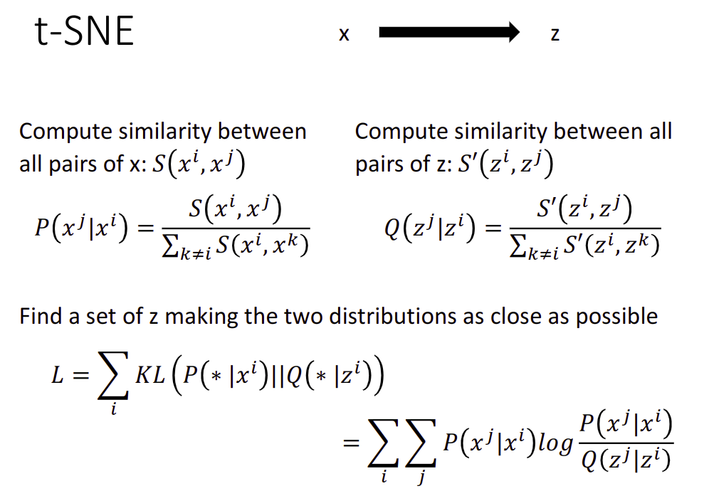

KL divergence
Similarity Measure
$S(x^i,x^j)=\exp (-||x^i-x^j||_ {2})$.
SNE: $S’(z^i,z^j$=\exp(-||z^i-z^j||_ 2)$.
t-SNE: $S’(z^i,z^j)=1/1+||z^i-z^j||_ 2$.

Unsupervised Learning: Deep Auto-encoder

Auto-encoder

找一个NN encoder和NNdecoder，将input转成一个code再转回成input，就可以两个连起来一起train
中间的是Bottleneck later
the auto-encoder can be deep

应用
文字处理
图片搜索
Pre-training DNN

变种
de-noising auto-encoder
contractive auto-endoer

Auto-endoer for CNN
CNN - unpooling
记录一下maxmap其他位置全补零，或全填最大值

CNN - Deconvolution
Actually, deconvolution is convolution

Unsupervised Learning - Deep Generative Model

Creation

generative model

PixelRNN

To Create an image, generating a pixel each time
It difficult to evaluate generation.

Variational Autoencoder (VAE)

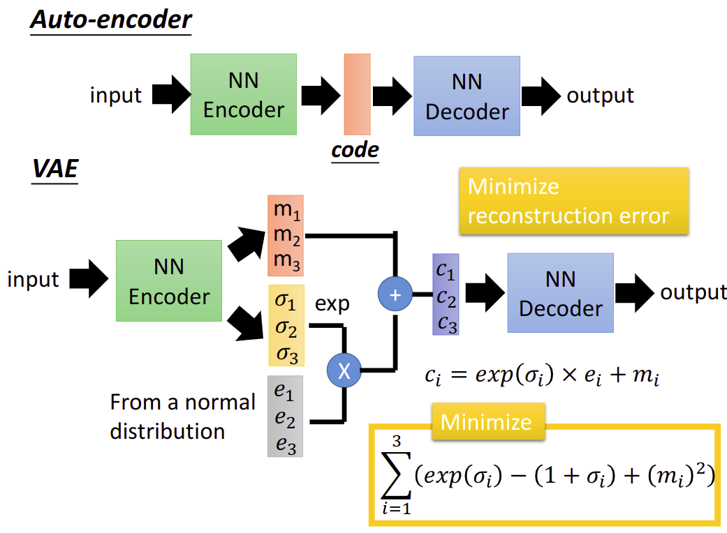
$m$是原来的encoder orginal code
$c$是noise
$\sigma$是The variance of noise is automatically learned
$e$是从normal distribution sample出来的值
注意要minimize的东西，如果不加前面的可能$\sigma$就是0了，让$\sigma$接近0，variance接近1

Why VAE？
Estimate the probability distribution.
用的方法就是Gasussian Mixture Model
$P(x)=\sum_{m} P(m)P(x|m)$.
$m\sim P(m)\text{(multinomial), m is a integer}$.
$x|m\sim N(\mu^m,\Sigma^m)$.
Each x you generate is from a mixture.
Distributed representation is better than cluster.
$z\sim N(0,I)$. $z$ is a vector from normal distribution.
$x|z\sim N(\mu(z),\sigma(z))$. Each dimension of $z$ represents an attribute. $\mu(z),\sigma(z)$ is going to be estimated, 可以用Neural Network来找这个function
$P(x)=\int_{z}P(z)P(x|z)\text{d}z$.
$L=\sum_{z}\log P(x)$. Maximizing the likelihood of the observed $x$.
Tuning the parameters to maximize likelihood $L$.
Another distribution $q(z|x)$，$z|x=N(\mu’(x),\sigma’(x))$. 这是一个相反的Network，这是VAE的encoder，上面的是decoder

Maximizing Likelihood
$P(x)=\int_{z}P(z)P(x|z)\text{d}z$.
$L=\sum_{z}\log P(x)$
$\log P(x)=\int_{z}q(z|x)\log P(x)\text{d}z=\int_{z}q(z|x)\log\left (\frac{P(z,x)}{P(z|x)}\right )\text{d}z$. $q(z|x)$ can be any distribution
$=\int_{z}q(z|x)\log\left( \frac{P(z,x)}{q(z|x)}\frac{q(z|x)}{P(z|x)} \right )\text{d}z$.
$=\int_{z}q(z|x)\log\left ( \frac{P(z,x)}{q(z|x)}\right )\text{d}z+\int_{z}q(z|x)\log\left ( \frac{q(z|x)}{P(z|x)}\right )\text{d}z$. 最后一项，是KL divergence, $KL(q(z|x)|| P(z|x)) \geqslant 0$
$\geqslant \int_{z}q(z|x)\log \left( \frac{P(x|z)P(z)}{q(z|x)}\right )$. lower bound $L_b$，就是上一行的第一项
所以
$\log P(x)=L_b+KL(q(z|x)||P(z|x))$.
$L_b=\int_{z}q(z|x)\log \left (\frac{P(x|z)P(z)}{q(z|x)} \right )\text{d}z$. Find $P(x|z)$ and $q(z|x)$ maximizing $L_b$.
$q(z|x)$ will be an approximation of $P(z|x)$ in the end.
$L_b=\int_{z}q(z|x)\log \left (\frac{P(x|z)P(z)}{q(z|x)} \right )\text{d}z$.
$=\int_{z}q(z|x)\log P(x|z)\text{d}z+\int_{z}q(z|x)\log \left ( \frac{P(z)}{q(z|x)}\right )\text{d}z$. $KL(q(z|x) || P(z))$.
Minimizing $KL(q(z|x)||P(z))$, $q(z|x)$是在一个Neural Network里面的，这个相当于VAE中Minimize $\sum{i=1}^{3}(\exp (\sigma_i)-(1+\sigma_i)+(m_i)^2)$.
Maximizing $\int_{z}q(z|x)\log P(x|z)\text{d}z=E_{q(z|x)}[\log P(x|z)]$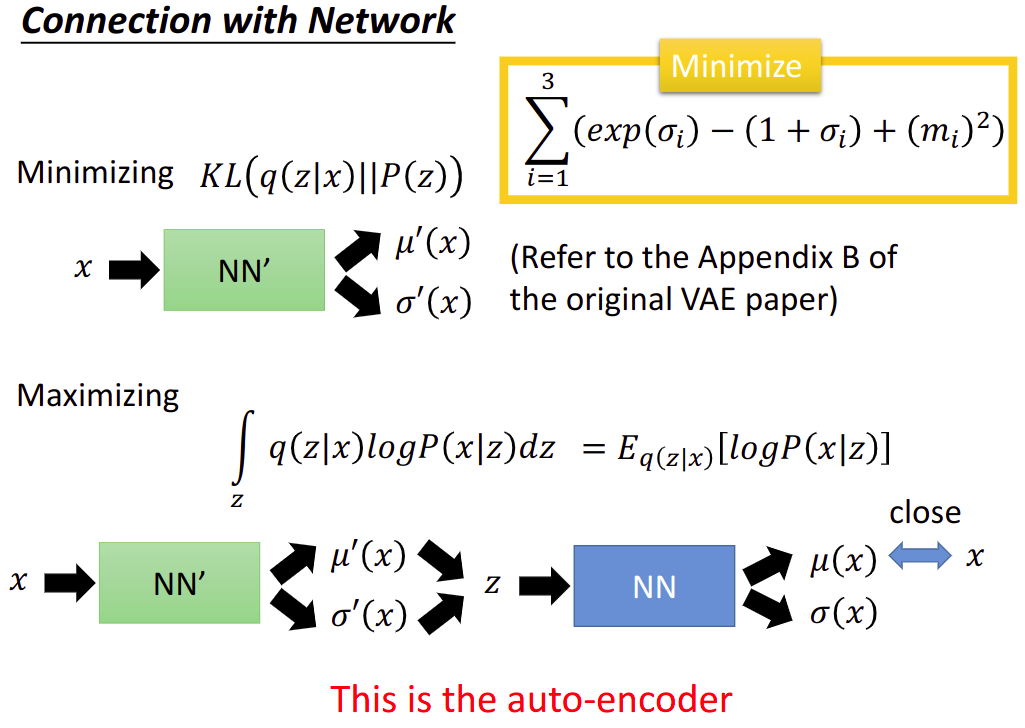

这是Auto-encoder做的事情，让输入和输出越接近越好.

Conditional VAE
抽出特征生成风格的图片

Problem of VAE
It does not really try to simulate real images.
VAE may just memorize the existing images, instead of generating new images.

Generative Adversarial Network (GAN)

最早论文 Ian J. Good fellow,Jean Pouget-Abadie,Mehdi Mirza,Bing Xu,David Warde-Farley,Sherjil Ozair,Aaron Courville,Yoshua Bengio, Generative Adversarial Networks, arXivpreprint 2014

GAN 分为两个部分，Generator 和 Discriminator.
Generator从未看过real data，来生成一组图片
Discriminator看过，它来做一个二元分类的问题，来判断Generator生成的data是否是real data(real or fake)
这时候再来train generator， “Tuning” the parameters of generator，希望让 The output be classified as “real” (as close to 1 as possible)，这时候也要让Discriminator的参数fix保持不变，以此往复。

目前存在的问题就是，可以骗过Discriminator的图片，不一定是真的图片，可能是一些奇怪的东西
还有就是Generator可能太弱，却依然可以骗过Discriminator

Transfer Learning

Transfer Learning 迁移学习
Data not directly related to the task considered.

Why? 一般原因都是数据难收集比较少之类的

Target Data是我们真正要的Data，Source Data是没有直接关系的Data
根据有无label分为4种情况，分别用对应的方法

Model Fine-tuning

Task description
- Target data: $(x^t, y^t)$. Very little
- Source data: $(x^s, y^s)$. A large amount
  One-shot learning: only a few examples in target domain
Example: (supervised) speaker adaption
- Target data: audio data and its transcriptions of specific user
- Source data: audio data and transcriptions from many speakers
Idea: training a model by source data, then fine-tune the model by target data
Challenge: only limited target data, so be careful about overfitting

Conservative Training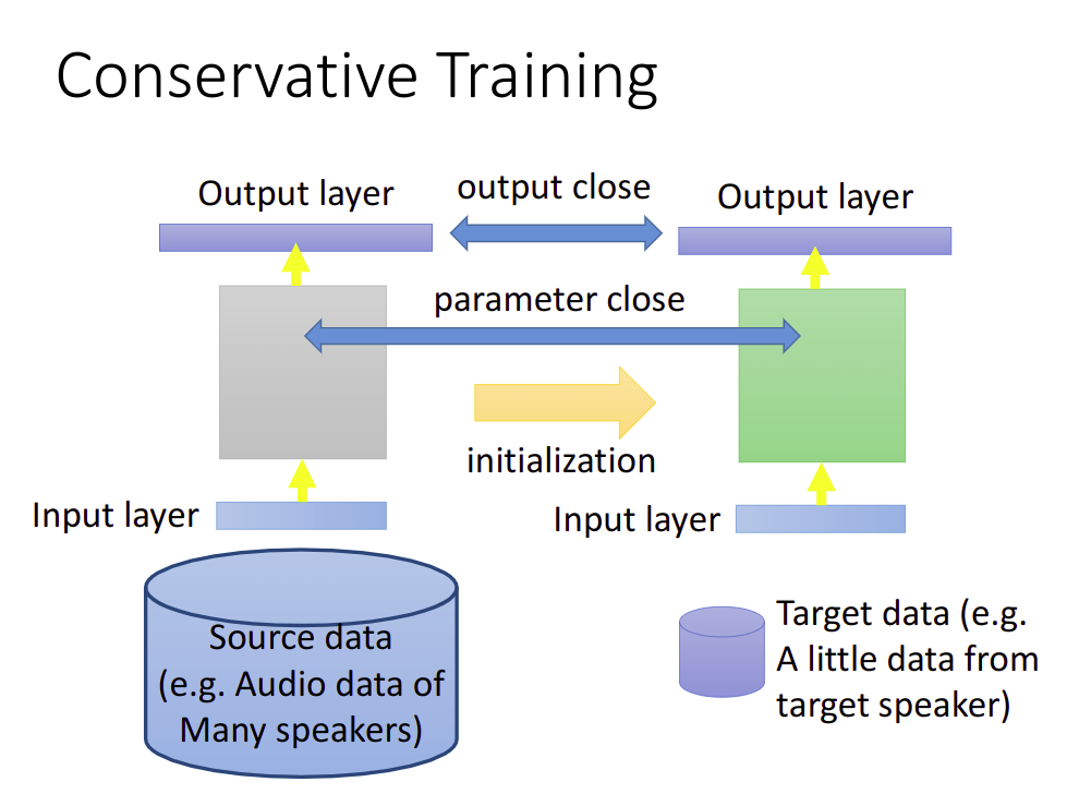

让两个Model的output相近

Layer Transfer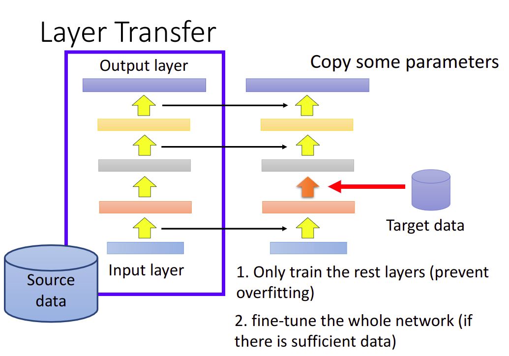

把几个Layer直接copy，光去train没有被copy的Layer，考虑的参数比较少
Which layer can be transferred (copied)?

Speech: usually copy the last few layers
Image: usually copy the first few layers

Multitask Learning

The multi-layer structure makes NN suitable for multitake learning.
不同的task有几个相同的Layer共用

常用的方向就是多语言辨识

Progressive Neural Networks

Domain-adversarial training

Task description

Source data: $(x^s, y^s)$. Training Data.
Target data: $(x^t)$. Testing Data. They are mismatched.

Similar to GAN. 需要通过一个Domain classifier.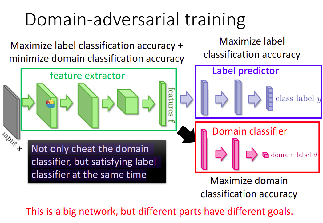

训练过程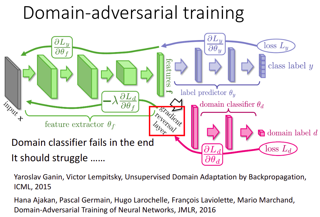

Zero-shot Learning

Task description

Source data: $(x^s, y^s)$. Training Data.
Target data: $(x^t)$. Testing Data. They are different tasks.

具体就是把Attribute embedding，然后在查database，让一个物品的图和他这类物品的attribute接近，两个function投影到embedding space上，也就是两个NN投影后的结果越接近越好。

Training Target: $f(x^n)$ and $g(y^n)$ as close as possible.

What if we don’t have database ? 换Attribute成Word vector.

$f^{\ast}, g^{\ast}=\arg \min_ {f,g}\sum_{n} || f(x^n)-g(y^n) ||_ {2}$. 这样是不行的，需要修改成下面的样子
$f^{\ast}, g^{\ast}=\arg \min_ {f,g}\sum_{n} \max (0, k-f(x^n)\cdot g(y^n) + \max_ {m\neq n} f(x^n)\cdot g(y^m)), k\text{ Margin you define}$.
Zero Loss: $k-f(x^n)\cdot g(y^n) + \max_ {m\neq n} f(x^n)\cdot g(y^m) < 0$.
$f(x^n)\cdot g(y^n) - \max_ {m\neq n} f(x^n)\cdot g(y^m)>k$. 把相对应的接近，不相对应的拆散

Convex Combination of Semantic Embedding

Example 就是语言的翻译，可以翻译一个从未见过的翻译方向，但翻译的两个语言都有其他语言翻译过

Support Vector Machine(SVM)

Hinge Loss + Kernel Method = Support Vector Machine(SVM) 支持向量机

Hinge Loss

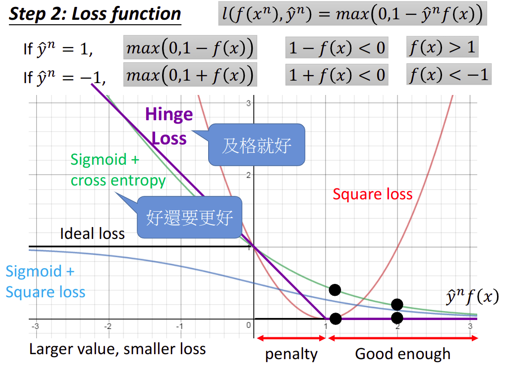
Hinge Loss就是最上面的那个Loss Function $l(f(x^n), \hat{y}^n)=\max (0, 1-\hat{y}^nf(x^n))$

Linear SVM

Step1: Function(Model)
$f(x)=\sum_{i}w_ix_i+b=\begin{bmatrix}w\\ b\end{bmatrix}\cdot \begin{bmatrix}x\\ 1\end{bmatrix}=w^{T}x$.
这里把第一个向量看成新的$w$，第二个向量看成是$x$.

Step2: Loss Function
$L(f)=\sum_{n}l(f(x^n), \hat{y}^n)+\lambda \begin{Vmatrix}w\end{Vmatrix}_ 2$.
$l(f(x^n), \hat{y}^n)=\max (0, 1-\hat{y}^nf(x^n))$.
是一个convex function

Step3: Gradient Descent
$\frac{\partial l(f(x^n), \hat{y}^n)}{\partial w_i}=\frac{\partial l(f(x^n), \hat{y}^n)}{\partial f(x^n)}\frac{\partial f(x^n)}{\partial w_i}$.
因为$f(x^n)=w^{T}\cdot x^n$.后面那项的值自然就是$x^n_i$.
而前面那项
$\frac{\partial \max(0, 1-\hat{y}^nf(x^n))}{\partial f(x^n)}=\left\{\begin{matrix}-\hat{y}^n, & \hat{y}^nf(x^n)<1 \text{or}1-\hat{y}^nf(x^n)>0\\ 0, & \text{otherwise}\end{matrix}\right.$.
$\frac{\partial L(f)}{\partial w_i}=\sum_{n}-\delta(\hat{y}^nf(x^n)<1)\hat{y}^nx^n_i$.

Another formulation
$L(f)=\sum_{n}\varepsilon ^n+\lambda \begin{Vmatrix}w\end{Vmatrix}_ 2,\varepsilon^n=\max(0,1-\hat{y}^nf(x))$.
$\varepsilon ^n\geqslant 0, \varepsilon ^n\geqslant 1-\hat{y}^nf(x)\rightarrow \hat{y}^nf(x)\geqslant 1-\varepsilon^n$.
因为要minimize Loss，所以下面这个$\varepsilon^n$的表示形式和上面的是相同的.
$\varepsilon ^n$: slack variable. Quadratic Programming(QP) Problem.

Dual Representation

Kernel Method
Step1:
$w^{\ast}=\sum_{n}a^{\ast}_ n x^n$. Linear combination of data points.
Hinge Loss的时候，$\alpha$是sparse的，有很多为0
所以写成向量形式$w=\sum_{n}a_n x^n=X\alpha$.
$f(x)=w^{T}x=\alpha^{T}X^{T}x$. 最后得到的就是一个scalar
$f(x)=\sum_{n}\alpha_n(x^n\cdot x)=\sum_{n}\alpha_{n}K(x^n,x)$. $K(x^n,x)$就是Kernel Function,是$x^n$和$x$的inner product.
Step2,3: Find $\{\alpha_1^{\ast},\alpha_2^{\ast},\cdots, \alpha_N^{\ast}\}$.
We don’t really need to know vector $x$.
We only need to know the inner project between a pair of vectors $x$ and $z$. $K(x,z)$. Kernel Trick

Directly computing $K(x,z)$ can be faster than “feature transformation + inner product” sometimes.
就是直接计算$K(x,z)$，可能要比eature transformation + inner product计算快上许多
比如$K(x,z)=\phi(x)\cdot \phi(z)=(x\cdot z)^2$.

Radial Basic Function Kernel
$K(x,z)=\exp \left ( -\frac{1}{2}\begin{Vmatrix}x-z\end{Vmatrix}_ 2\right )=\phi (x)\cdot \phi (z)$. $\phi (\ast)$ has inf dim.
$=\exp \left ( -\frac{1}{2}\begin{Vmatrix}x\end{Vmatrix}_ 2-\frac{1}{2}\begin{Vmatrix}z\end{Vmatrix}_ 2+x\cdot z\right )$.
$=\exp \left(-\frac{1}{2}\begin{Vmatrix}x\end{Vmatrix}_ 2 \right )\exp \left(-\frac{1}{2}\begin{Vmatrix}z\end{Vmatrix}_ 2 \right )\exp(x\cdot z)=C_xC_z\exp (x\cdot z)=C_xC_z\sum_{i=0}^{\infty}\frac{(x\cdot z)^i}{i!}$. Tayor展开

Sigmoid Kernel
$K(x,z)=\tanh (x\cdot z)$.
When using sigmoid kernel, we have a 1 hidden layer network.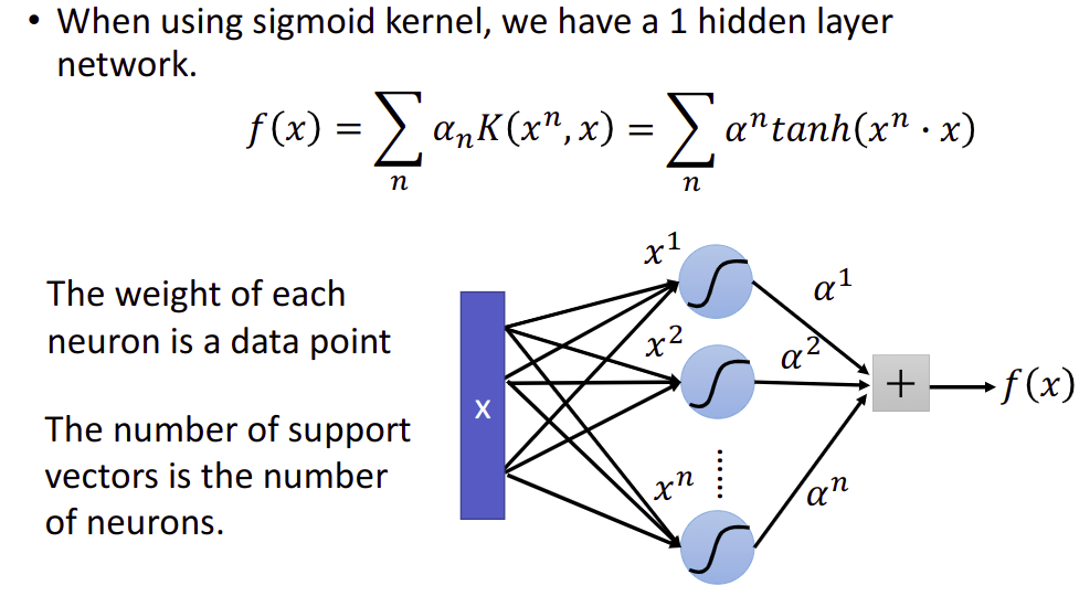

You can directly design $K(x,z)$ instead of considering $\phi (x), \phi (z)$.
When $x$ is structured object like sequence, hard to design $\phi(x)$.
$K(x,z)$ is something like similarity. (Mercer’s theory can check)

Recurrent Neural Network

一种有记忆的NN，可以根据上下文判断的NN

The output of hidden layer are stored in the memory.
Memory can be considered as another input.

All the weights are “1”, no bias.
All activation functions are linear

Changing the sequence order will change the output.

Elman Network. 就是每层的output当成这层的input
Jordan Network. 最后的output当成input

Bidirectional RNN

双向的RNN，扩大看到的范围，不仅可以从上文还可以从下文看

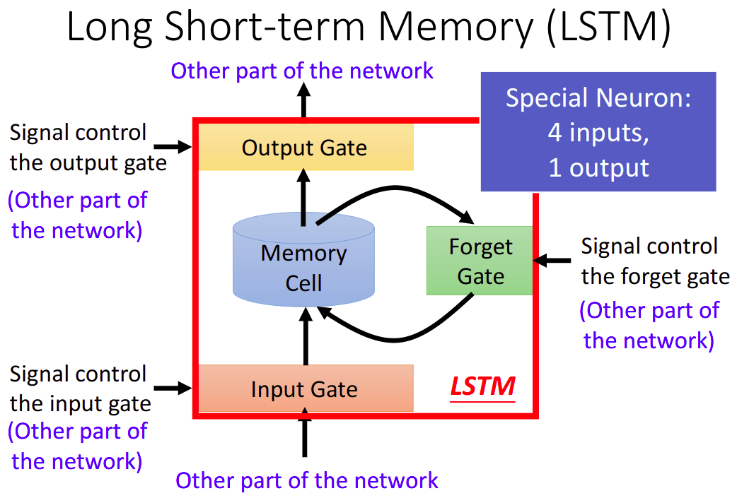
Long Short-term Memory(LSTM)

这三个参数，是根据输入的vector的transpose得到的

Learning

用的也是Gradient Descent，但是是一种Backpropagation through time(BPTT)

RNN也是比较难Train的
The error surface is rough.
RNN的Total Loss是非常陡峭的，Error Surface有些地方非常平坦，有些地方非常陡峭
有个方法就是Clipping，当Gradient超过某一个值的时候，就等于这个值，也就是设置个上限，不至于参数飞出去

Helpful Techniques

Long Short-term Memory(LSTM)

Can deal with gradient vanishing(not gradient explode).
Memory and input are added.
The influence never disappears unless forget gate is closed.

Gated Recurrent Unit(GRU)

Clockwise RNN
Structurally Constrained Trcurrent Network(SCRN)
Vanilla RNN Initialized with Identity matrix + ReLU activation function.

More Application

Many to One : Input is a vector sequence, but output is only one vector

Sentiment Analysis
Key Term Extraction

Many to Many : Both input and output are both sequences, but the output is shorter.

Speech Recognition
但是这个，在每一小段时间中识别，最后去除重复的不能识别叠字
Connectionist Temporal Classification(CTC)
在之间可以添加符号null，可以解决叠字问题
Sequence to sequence learning
Both input and output are both sequences with different lengths.
比如做Machine Translation
Beyond Sequence
Syntactic parsing
Sequence-to-sequence Auto-encoder - Text
To understand the meaning of a word sequence, the order of the words can not be ignored.
Sequence-to-sequence Auto-encoder - Speech
Dimension reduction for a sequence with variable length audio segments(word-level) -> fixed-length vector

Attention-based Model

Reading Head Controller
Writing Head Controller

Neural Turing Machine

常用在Reading Comprehension

Integrated Together

deep learning和structured learning结合起来。input features 先通过RNN/LSTM，然后RNN/LSTM的output再做为HMM/svm的input。用RNN/LSTM的output来定义HMM/structured SVM的evaluation function，如此就可以同时享有deep learning的好处，也可以有structure learning的好处。

下面讨论了一下structure Learning是否practical的问题

Ensemble

集成学习

Framework of Ensemble

Get a set of classifiers. They should be diverse.
Aggregate the classifiers(properly).

就是多个model一起搞的感觉

Bagging

将几个model的结果平均，这样如果你的model非常复杂，很容易overfit那么这是很有效的，因为bias比较小，variance比较大。

Decision Tree 就比较容易overfit，需要做bagging
这个就简单讲了一下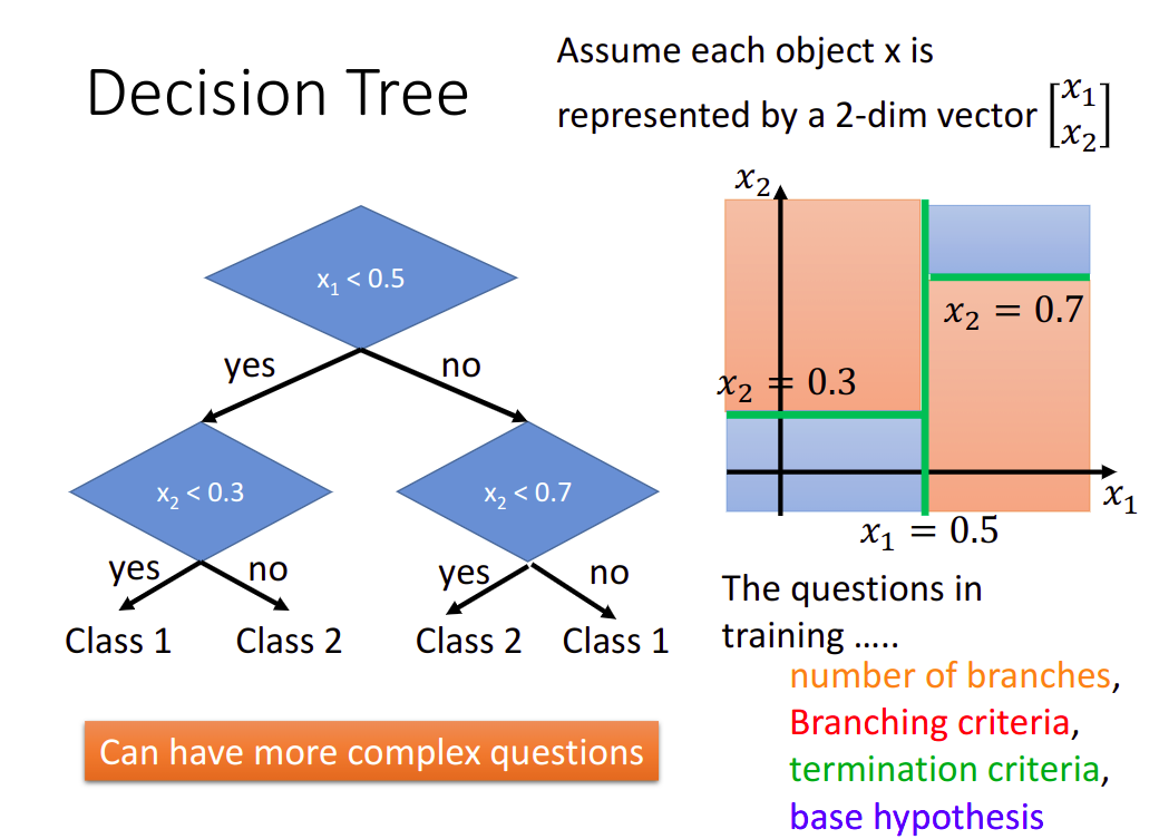

Random Forest

Descision Tree is easy to achieve 0% error rate on training data, if each training example has its own leaf..
Random forest: Bagging of decision tree

Resampling trainging data is not sufficient.
Randomly restrict the features/questions used in each split.
Out-of-bag validation for bagging

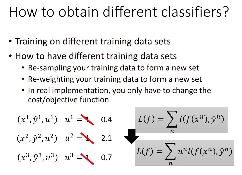
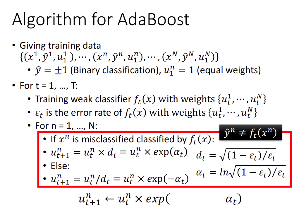
Boosting

Improving Weak Classifiers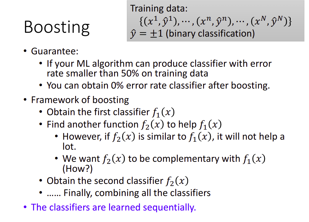

其中最经典的一个做法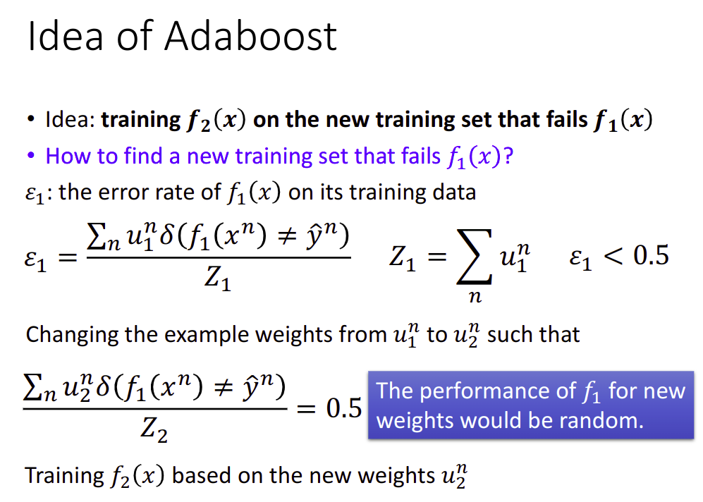

Math Warning，说实话这段没打听懂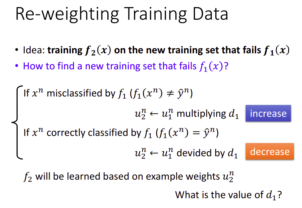

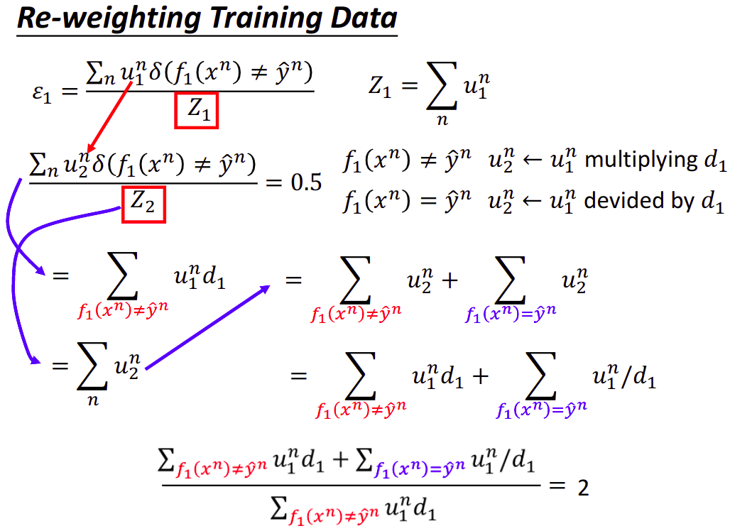
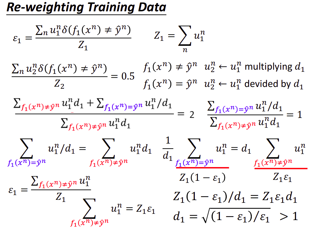
这张图片里的空白在下张图片中出现了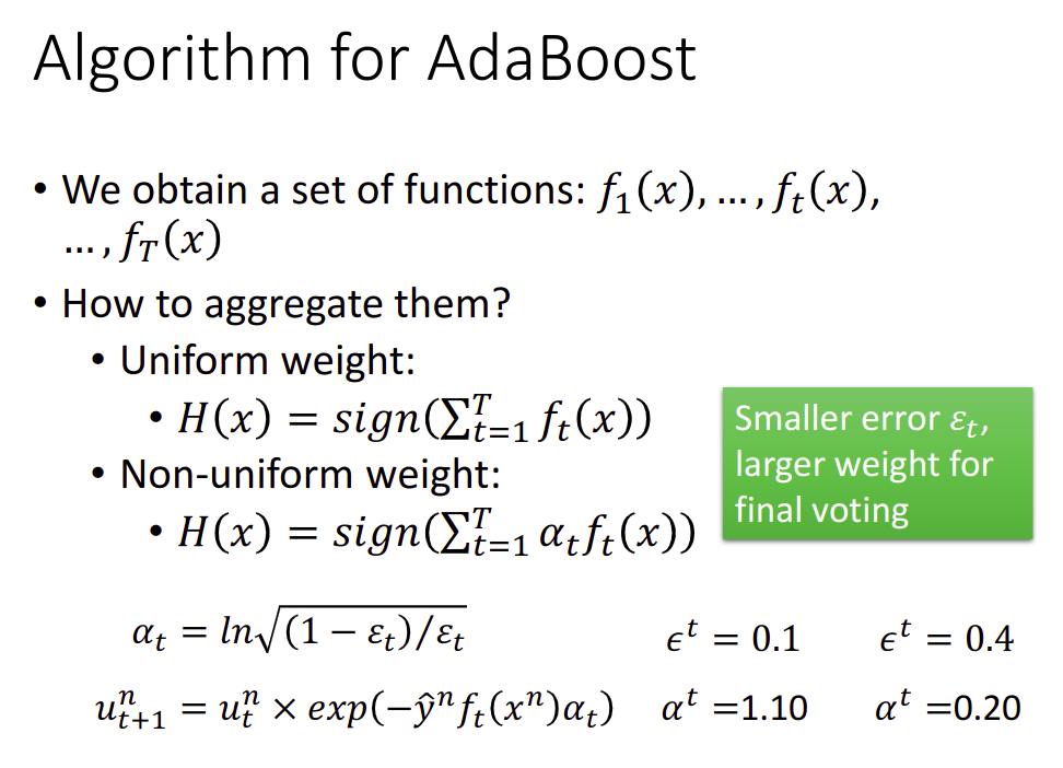

证明地方真的晕了，改天看8…

Stacking

Majority Vote

Deep Reinforcement Learning

这里就略讲了一下
主要是几个部分
Environment->observation/state & reward -> Agent -> action -> Environment
要做的就是maximize reward

难点
Reward delay
Agent’s actions affect the subsequent data it receives

方法
就是Policy-based 和Value-based
先有Valued-based的方法，再有Policy-based的方法。在Policy-based的方法里面，会learn一个负责做事的Actor，在Valued-based的方法会learn一个不做事的Critic，专门批评不做事的人。我们要把Actor和Critic加起来叫做Actor+Critic的方法。
Asynchronous Advantage Actor-Critic(A3C)这个方法比较强

reference